The ADALINE - Theory and Implementation of the First Neural Network Trained With Gradient Descent

10 Mar 2020

Share this:

Learning objectives

Understand the principles behind the creation of the ADALINE
Identify the similarities and differences between the perceptron and the ADALINE
Acquire an intuitive understanding of learning via gradient descent
Develop a basic code implementation of the ADALINE in Python
Determine what kind of problems can and can’t be solved with the ADALINE

Historical and theoretical background

The ADALINE (Adaptive Linear Neuron) was introduced in 1959, shortly after Rosenblatt’s perceptron, by Bernard Widrow and Ted Hoff (one of the inventors of the microprocessor) at Stanford. Widrow and Hoff were electrical engineers, yet Widrow had attended the famous Dartmouth workshop on artificial intelligence in 1956, an experience that got him interested in the idea of building brain-like artificial learning systems. When Widrow moved from MIT to Stanford, a colleague asked him whether he would be interested in taking Ted Hoff as his doctoral student. Widrow and Hoff came up with the ADALINE idea on a Friday during their first session working together. At the time, implementing an algorithm in a mainframe computer was slow and expensive, so they decided to build a small electronic device capable of being trained by the ADALINE algorithm to learn to classify patterns of inputs.

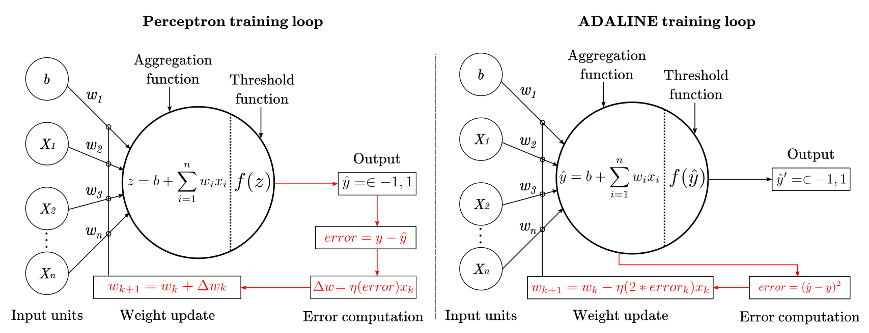
The main difference between the perceptron and the ADALINE is that the later works by minimizing the mean squared error of the predictions of a linear function. This means that the learning procedure is based on the outcome of a linear function rather than on the outcome of a threshold function as in the perceptron. Figure 2 summarizes such difference schematically.

From a cognitive science perspective, the main contribution of the ADALINE was methodological rather than theoretical. Widrow and Hoff were not primarily concerned with understanding the organization and function of the human mind. Although the ADALINE was initially applied to problems like speech and pattern recognition (Talbert et al., 1963), the main application of the ADALINE was in adaptive filtering and adaptive signal processing. Technologies like adaptive antennas, adaptive noise canceling, and adaptive equalization in high-speed modems (which makes Wifi works well), were developed by using the ADALINE (Widrow & Lehr, 1990).

Mathematically, learning from the output of a linear function enables the minimization of a continuous cost or loss function. In simple terms, a cost function is a measure of the overall badness (or goodness) of the network predictions. Continuous cost functions have the advantage of having “nice” derivatives, that facilitate training neural nets by using the chain rule of calculus. This change opened the door to train more complex algorithms like non-linear multilayer perceptrons, logistic regression, support vector machines, and others.

Next, we will review the ADALINE formalization, learning procedure, and optimization process.

Mathematical formalization

Mathematically, the ADALINE is described by:

a linear function that aggregates the input signal
a learning procedure to adjust connection weights

Depending on the problem to be approached, a threshold function, as in the McCulloch-Pitts and the perceptron, can be added. Yet, such function is not part of the learning procedure, therefore, it is not strictly necessary to define an ADALINE.

Linear aggregation function

The linear aggregation function is the same as in the perceptron:

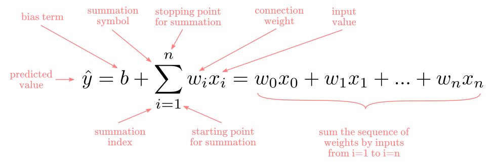
For a real-valued prediction problem, this is enough.

Threshold decision function

When dealing with a binary classification problem, we will still use a threshold function, as in the perceptron, by taking the sign of the linear function as:

$\hat{y}' = f(\hat{y}) = \begin{cases} +1, & \text{if } \hat{y}\ \text{> 0} \\ -1, & \text{otherwise} \end{cases}$

where $\hat{y}$ is the output of the linear function.

The Perceptron and ADALINE fundamental difference

If you read my previous article about the perceptron, you may be wondering what’s the difference between the perceptron and the ADALINE considering that both end up using a threshold function to make classifications. The difference is the learning procedure to update the weight of the network. The perceptron updates the weights by computing the difference between the expected and predicted class values. In other words, the perceptron always compares +1 or -1 (predicted values) to +1 or -1 (expected values). An important consequence of this is that perceptron only learns when errors are made. In contrast, the ADALINE computes the difference between the expected class value $y$ (+1 or -1), and the continuous output value $\hat{y}$ from the linear function, which can be any real number. This is crucial because it means the ADALINE can learn even when no classification mistake has been made. This is a consequence of the fact that predicted class values $\hat{y}’$ do not influence the error computation. Since the ADALINE learns all the time and the perceptron only after errors, the ADALINE will find a solution faster than the perceptron for the same problem. Figure 1 illustrate this difference in the paths and formulas highlighted in red.

Figure 1

The ADALINE error surface

Before approaching the formal definition of the ADALINE learning procedure, let’s briefly explore what does it mean to “minimize the mean of the sum of squared errors”. If you are familiar with the least-squares method in regression analysis, this is exactly the same. You can skip to the next section if you feel confident about it.

In a single iteration, the error in the ADALINE is calculated as $(y - \hat{y})^2$, in words, by squaring the difference between the expected value and the predicted value. This process of comparing the expected and predicted values is repeated for all cases, $j=1$ to $j=n$, in a given dataset. Once we add the squared difference for the entire dataset and divide by the total, we obtained the so-called mean of squared errors (MSE). Formally:

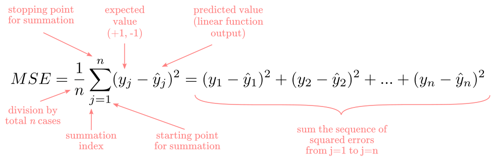
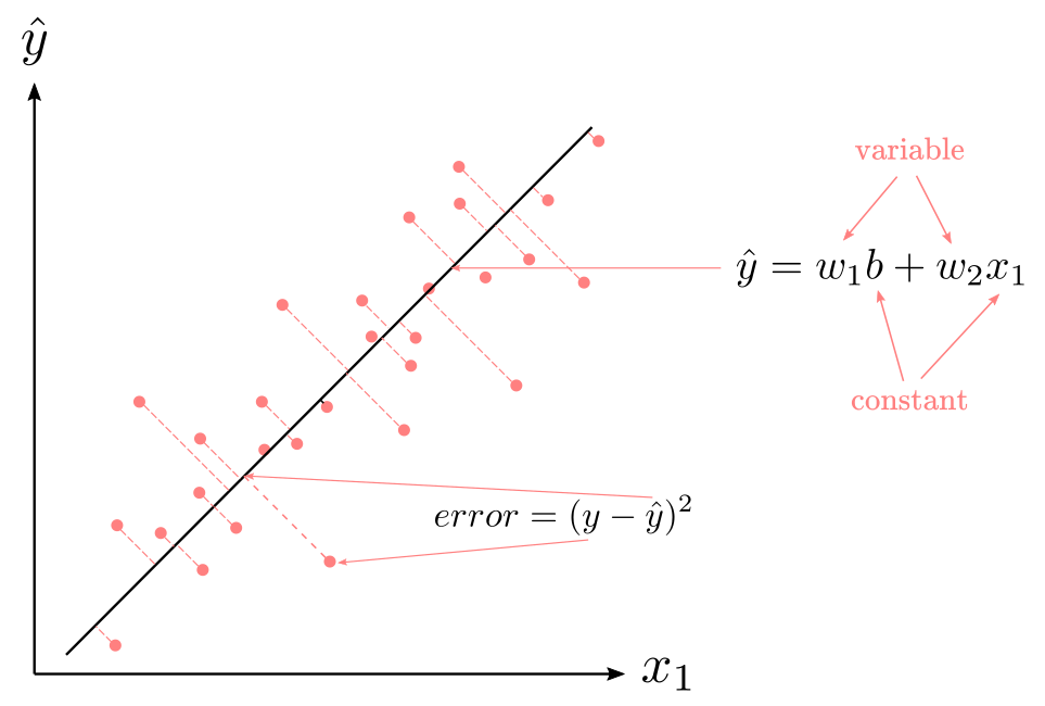
Figure 2 shows a visual example of the least-squares method with one predictor. The horizontal axis represents the $x_1$ predictor (or feature), the vertical axis represents the predicted value $\hat{y}$, and the pinkish dots represent the expected values (real data points). If you remember your high-school algebra, you may know that $\hat{y}=w_1b+w_2x_1$ defines a line a cartesian plane. They key, is that the intercept (i.e., where the line begins) and the slope (i.e., degree of inclination) of the line is determined by the $w_1$ and $w_2$ weights. The $b$ and $x_1$ values are given, do not change, therefore, they can’t influence the shape of the line.

Figure 2

The goal of the least-squares algorithm is to generate as little cumulative error as possible. This equals to find the line that best fit the points in the cartesian plane. Since the weights are the only values we can adjust to change the shape of the line, different pairs of weights will generate different means of squared errors. This is our gateway to the idea of finding a minima in an error surface. Imagine the following: you are trying to find the set of weights, $w_1$ and $w_2$ that would generate the smallest mean of squared error. Your weights can take values ranging from 0 to 1, and your error can go from 0 to 1 (or 0% to 100% thinking proportionally). Now, you decide to plot the mean of squared errors against all possible combinations of $w_1$ and $w_2$. Figure 3 shows the resulting surface:

Figure 3

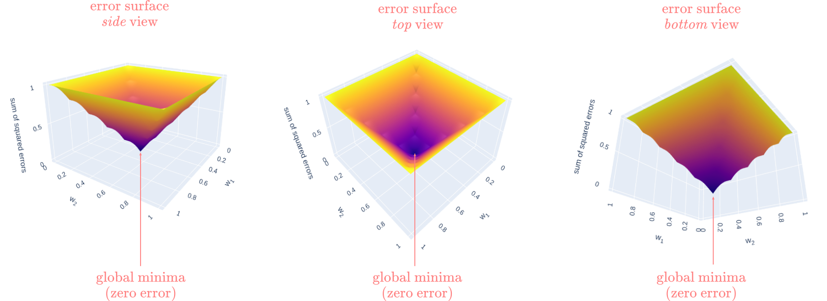
We call this an error surface. In this case, the shape of the error surface is similar to a cone or pyramid with -crucially- a single point where the error goes all the way down to zero at the bottom of the object. In mathematics, this point is known as global minima. This type of situation, when a unique set of weights defines a single point where the error is zero, is known as a convex optimization problem. If you try this document in interactive mode (mybinder or locally), you can run the code below and play with the interactive 3D cone (remove the # symbols and run the cell to see the plot).

import plotly.graph_objs as go
import numpy as np

x = np.arange(0,1.1,0.1)
y = np.arange(0,1.1,0.1)
z = [
    [1, 1, 1, 1, 1, 1, 1, 1, 1, 1, 1],
    [1,.8,.8,.8,.8,.8,.8,.8,.8,.8, 1],
    [1,.8,.6,.6,.6,.6,.6,.6,.6,.8, 1],
    [1,.8,.6,.4,.4,.4,.4,.4,.6,.8, 1],
    [1,.8,.6,.4,.2,.2,.2,.4,.6,.8, 1],
    [1,.8,.6,.4,.2,.0,.2,.4,.6,.8, 1],
    [1,.8,.6,.4,.2,.2,.2,.4,.6,.8, 1],
    [1,.8,.6,.4,.4,.4,.4,.4,.6,.8, 1],
    [1,.8,.6,.6,.6,.6,.6,.6,.6,.8, 1],
    [1,.8,.8,.8,.8,.8,.8,.8,.8,.8, 1],
    [1, 1, 1, 1, 1, 1, 1, 1, 1, 1, 1]
]

fig = go.Figure(go.Surface(x=x, y=y, z=z))

scene = dict(xaxis_title='w<sub>1</sub>',
             yaxis_title='w<sub>2</sub>',
             zaxis_title='mean of squared errors',
             aspectratio= {"x": 1, "y": 1, "z": 0.6},
             camera_eye= {"x": 1, "y": -1, "z": 0.5})

####~~~ Uncomment in binder or locally to see 3D plot ~~~~####

# fig.layout.update(scene=scene,
#                    width=700,
#                    margin=dict(r=20, b=10, l=10, t=10))


# fig.show()

All neural networks can be seen as solving optimization problems, usually, in high-dimensional spaces, with thousands or millions of weights to be adjusted to find the best solution. AlexNet, the model that won the ImageNet Visual Recognition Challenge in 20212, has 60,954,656 adjustable parameters. Nowadays, in 2020, most state-of-the-art neural networks have several orders of magnitude more parameters than AlexNet.

Alas, the bad news is that most problems worth solving in cognitive science are nonconvex, meaning that finding the so-called global minima becomes extremely hard, and in most cases can’t be guaranteed. In the 3D case, instead of having a nice cone-like error surface, we obtain something more similar to a complex landscape of mountains and valleys, like the Cordillera de Los Andes or the Rocky Mountains. Figure 4 shows an example of such a landscape:

Figure 4

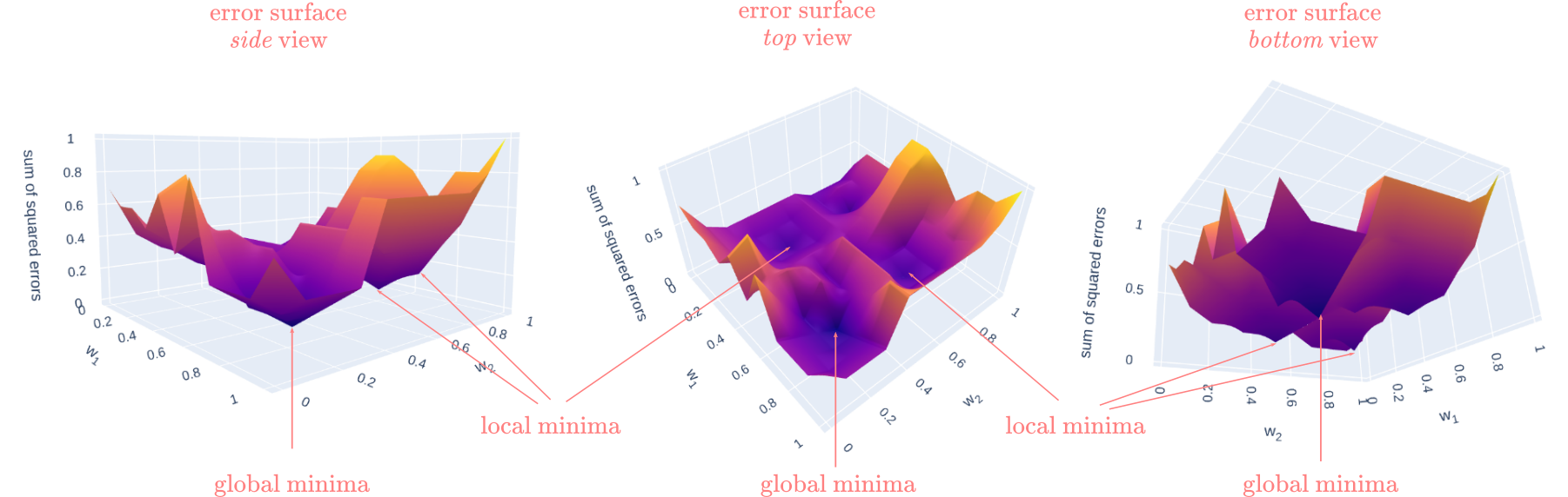
Now, instead of having a unique point where the error is at its minimum, we have multiple low points or “valleys” at different sections in the surface. Those “valleys” are called local minima, or the point of minimum error for that section. Ideally, we always want to find the “global minima”, yet, with a landscape like this, finding it may become very hard and slow. If you try this document in interactive mode (mybinder or locally), you can run the code below and play with the interactive 3D surface (remove the # symbols and run the cell to see the plot).

import plotly.graph_objs as go
import numpy as np

x = np.arange(0,1.1,0.1)
y = np.arange(0,1.1,0.1)
z = [
    [.7,.6,.6,.5,.7,.4,.8,.3,.3,.3,.5],
    [.4,.4,.4,.4,.8,.5,.4,.2,.2,.2,.3],
    [.3,.3,.3,.3,.3,.5,.1,.1,.1,.2,.3],
    [.3,.2,.2,.2,.3,.4,.4, 0,.1,.2,.3],
    [.3,.2,.1,.2,.3,.2,.2,.3,.4,.7,.7],
    [.3,.2,.2,.2,.3,.5,.5,.5,.5,.4,.7],
    [.3,.3,.3,.3,.3,.2,.2,.2,.2,.4,.7],
    [.2,.2,.2,.3,.4,.4,.2,.1,.2,.4,.7],
    [.2,.3,.1,.3,.6,.6,.2,.2,.2,.4,.7],
    [.2,.3,.3,.3,.8,.8,.4,.4,.4,.5,.8],
    [.3,.5,.5,.5,.9,.9,.8,.6,.8,.8, 1]
]

fig = go.Figure(go.Surface(x=x, y=y, z=z))

scene = dict(xaxis_title='w<sub>1</sub>',
             yaxis_title='w<sub>2</sub>',
             zaxis_title='mean of squared errors',
             aspectratio= {"x": 1, "y": 1, "z": 0.6},
             camera_eye= {"x": 1, "y": -1, "z": 0.5})

####~~~ Uncomment in binder or locally to see 3D plot ~~~~####

# fig.layout.update(scene=scene,
#                   width=700,
#                   margin=dict(r=20, b=10, l=10, t=10))
#
# fig.show()

Learning procedure

By now, we know that we want to find a set of parameters that minimize the mean of squared errors. The ADALINE approaches this by utilizing the so-called gradient descent algorithm. For convex problems (cone-like error surface), gradient descent is guaranteed to find the global minima. For nonconvex problems, gradient descent is only guaranteed to find a local minimum, that may or may not be the global minima as well. At this point, we will only discuss convex optimization problems.

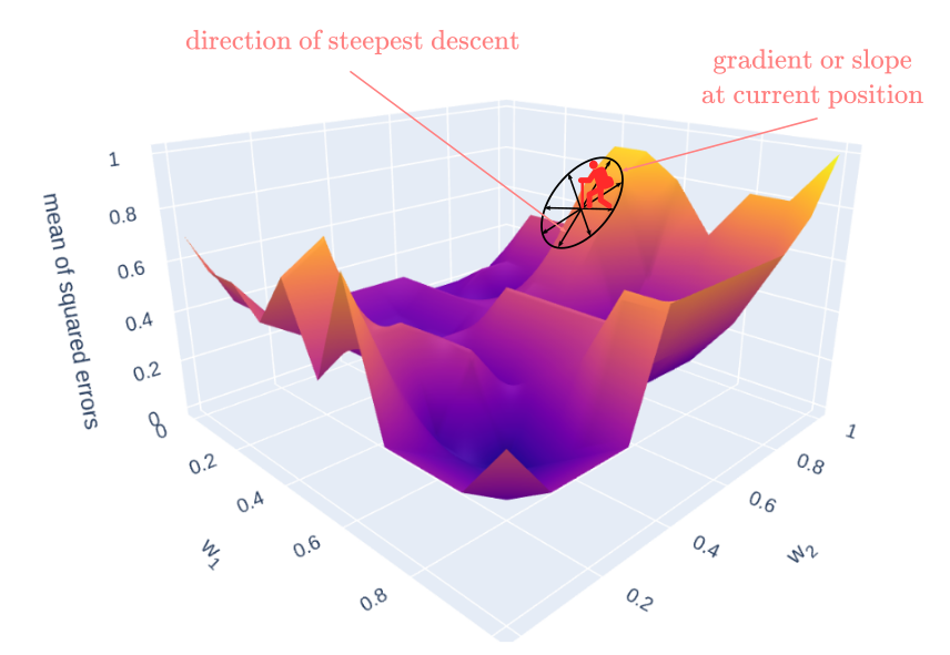
Imagine that you are hiker at the top of a mountain in the side of a valley. Similar to Figure 5. Your goal is to reach the base of the valley. Logically, you would want to walk downhill over the hillside until you reach the base. In the context of training neural networks, this is what we call “descending a gradient”. Now, it would be nice if you could do this efficiently, meaning to follow the path that will get you faster to the base of the valley. In gradient descent terms, this equals to move along the error surface in the direction where the gradient (degree of inclination) is steepest. As a hiker, you can visually inspect your surroundings to determine the best path. In an optimization context, we can use the chain-rule of calculus to estimate the gradient and adjust the weights.

Figure 5

For conciseness, let’s define the error of the network as function $E$.

$E(\hat{y}) = \frac{1} n\sum_{j=1}^{n}(y_j - \hat{y_j})^2$

If we expand $\hat{y_j}$, whe obtain:

$E(w,x) = \frac{1} n\sum_{j=1}^{n}(y_j - (b+\sum_{i}w_ix_i)_j)^2$

Now, remember that the only values we can adjust to change $\hat{y}$ are the weights, $w_i$. In differential calculus, taking derivatives means calculating the rate of change of a function with respect to an infinitely small change in an input argument. If “infinitely small” sounds like nonsense to you, for practical purposes, think about it as a very small change, let’s say, 0.000001. In our case, it means to compute the rate of change of the $E$ function in response to a very small change in $w$. That is what we call to compute a gradient, that we will call $\Delta$, at a point in the error surface.

Widrow and Hoff have the idea that instead of computing the gradient for the total mean squared error $E$, they could approximate the gradient’s value by computing the partial derivative of the error with respect to the weights on each iteration. Since we are dealing with a single case, let’s drop the summation symbols and indices for clarity. The function to derivate becomes:

$e(w,x) =(y-(b+wx))^2$

Now comes the fun part. By applying the chain-rule of calculus, the gradient of $e$:

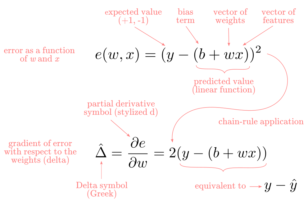
This may come as a surprise to you, but the gradient, in this case, is as simple as 2 times the difference between the expected and predicted value. Now we know the $\hat{\Delta}$ we need to update the weights at each iteration. Finally, the rule to update the weights says the following: “change the weight, $w_j$, by a portion, $\eta$, of the calculated negative gradient, $\Delta_j$”. We use the negative of the gradient because we want to go “downhill”, otherwise, you will be climbing the surface in the wrong direction. Formally, this is:

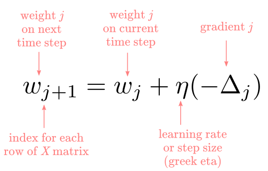
We use a portion ($\eta$) of the gradient instead of the full value to avoid “bouncing around” the minima of the function. This is easier to understand by looking at a simplified example as in Figure 6

Figure 6

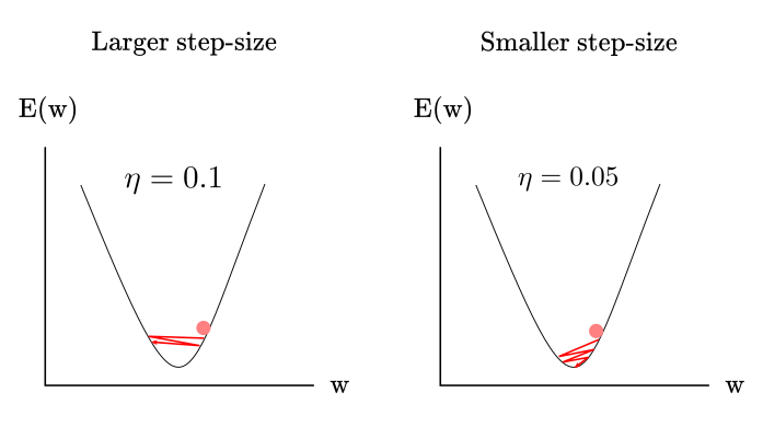
In the left pane, the value of $\eta$ is too large to allow the ball to reach the minima of the function so the ball “bounces around” the minima without reaching it. In the right pane, the value of $\eta$ is small enough to allow the ball to reach the minima after a few iterations. Adjusting the step-size or learning rate to find a minimum is usually solved by semi-automatically searching over different values of $\eta$ when training networks. “Why don’t use very small values of $\eta$ all the time?” Because there is a trade-off on training time. Smaller values of $\eta$ may help to find the minima, but it will also extend the training time as usually more steps are needed to find the solution.

Code implementation

We will implement the ADALINE from scratch with python and numpy. The goal is to understand the perceptron step-by-step execution rather than achieving an elegant implementation. I’ll break down each step into functions to ensemble everything at the end.

The first elements of the ADALINE are essentially the same as in the perceptron. Therefore, we could put those functions in a separate module and call the functions instead of writing them all over again. I’m not doing this to facilitate two things: to refresh the inner workings of the algorithm in code, and to provide with the full description for readers have not read the previous post. If you reviewed the perceptron post already, you may want to skip to the Training loop - Learning procedure section.

Generate vector of random weights

import numpy as np

def random_weights(X, random_state: int):
    '''create vector of random weights
    Parameters
    ----------
    X: 2-dimensional array, shape = [n_samples, n_features]
    Returns
    -------
    w: array, shape = [w_bias + n_features]'''
    rand = np.random.RandomState(random_state)
    w = rand.normal(loc=0.0, scale=0.01, size=1 + X.shape[1])
    return w

Predictions from the ADALINE are obtained by a linear combination of features and weights. This is the output of the linear aggregation function. It is common practice begining with a vector of small random weights that would be updated later by the perceptron learning rule.

Compute net input: linear aggregation function

def net_input(X, w):
    '''Compute net input as dot product'''
    return np.dot(X, w[1:]) + w[0]

Here we pass the feature matrix and the previously generated vector of random weights to compute the inner product. Remember that we need to add an extra weight for the bias term at the beginning of the vector (w[0)

Compute predictions: threshold function

def predict(X, w):
    '''Return class label after unit step'''
    return np.where(net_input(X, w) >= 0.0, 1, -1)

Remember that although ADALINE learning rule works by comparing the output of a linear function against the class labels when doing predictions, we still need to pass the output by a threshold function to get class labels as in the perceptron.

Training loop - Learning procedure

def fit(X, y, eta=0.001, n_iter=1):
    '''loop over exemplars and update weights'''
    mse_iteration = []
    w = random_weights(X, random_state=1)
    for pair in range(n_iter):
        output = net_input(X, w)
        gradient = 2*(y - output)
        w[1:] += eta*(X.T @ gradient)
        w[0] += eta*gradient.sum()
        mse = (((y - output)**2).sum())/len(y)
        mse_iteration.append(mse)
    return w, mse_iteration

Let’s examine the fit method that implements the ADALINE learning procedure:

Create a vector of random weights by using the random_weights function with dimensionality equal to the number of columns in the feature matrix
Loop over the entire dataset n_iter times with for pair in range(n_iter)
Compute the inner product between the feature matrix $X$ and the weight vector $w$ by using the net_input(X, w) function
Compute the gradient of error with respect to the weights 2*(y - output)
Update the weights in proportion to the learning rate $\eta$ by w[1:] += eta*(X.T @ gradient) and w[0] += eta*gradient.sum()
Compute the MSE mse = (((y - output)**2).sum())/len(y)
Save the MSE for each iterationmse_iteration.append(mse)

Application: classification using the peceptron

We will use the same problem as in the perceptron to test the ADALINE: classifying birds by their weight and wingspan. I will reproduce the synthetic dataset with two species: Wandering Albatross and Great Horned Owl. We are doing this to compare the performance of the ADALINE against the perceptron, which hopefully will expand our understanding of these algorithms.

One more time, I’ll repeat all the code to set up the classification problem, for the same reasons explained before. If you reviewed the perceptron chapter, you can skip these steps.

Generate dataset

Let’s first create a function to generate our synthetic data

def species_generator(mu1, sigma1, mu2, sigma2, n_samples, target, seed):
    '''creates [n_samples, 2] array
    
    Parameters
    ----------
    mu1, sigma1: int, shape = [n_samples, 2]
        mean feature-1, standar-dev feature-1
    mu2, sigma2: int, shape = [n_samples, 2]
        mean feature-2, standar-dev feature-2
    n_samples: int, shape= [n_samples, 1]
        number of sample cases
    target: int, shape = [1]
        target value
    seed: int
        random seed for reproducibility
    
    Return
    ------
    X: ndim-array, shape = [n_samples, 2]
        matrix of feature vectors
    y: 1d-vector, shape = [n_samples, 1]
        target vector
    ------
    X'''
    rand = np.random.RandomState(seed)
    f1 = rand.normal(mu1, sigma1, n_samples)
    f2 = rand.normal(mu2, sigma2, n_samples)
    X = np.array([f1, f2])
    X = X.transpose()
    y = np.full((n_samples), target)
    return X, y

According to Wikipedia, the wandering albatross mean weight is around 9kg (19.8lbs), and their mean wingspan is around 3m (9.8ft). I will generate a random sample of 100 albatross with the indicated mean values plus some variance.

albatross_weight_mean = 9000 # in grams
albatross_weight_variance =  800 # in grams
albatross_wingspan_mean = 300 # in cm
albatross_wingspan_variance = 20 # in cm 
n_samples = 100
target = 1
seed = 100

# aX: feature matrix (weight, wingspan)
# ay: target value (1)
aX, ay = species_generator(albatross_weight_mean, albatross_weight_variance,
                           albatross_wingspan_mean, albatross_wingspan_variance,
                           n_samples,target,seed )

import pandas as pd

albatross_dic = {'weight-(gm)': aX[:,0],
                 'wingspan-(cm)': aX[:,1], 
                 'species': ay,
                 'url': "https://raw.githubusercontent.com/pabloinsente/nn-mod-cog/master/notebooks/images/albatross.png"}

# put values in a relational table (pandas dataframe)
albatross_df = pd.DataFrame(albatross_dic)

According to Wikipedia, the great horned owl mean weight is around 1.2kg (2.7lbs), and its mean wingspan is around 1.2m (3.9ft). Again, I will generate a random sample of 100 owls with the indicated mean values plus some variance.

owl_weight_mean = 1000 # in grams
owl_weight_variance =  200 # in grams
owl_wingspan_mean = 100 # in cm
owl_wingspan_variance = 15 # in cm
n_samples = 100
target = -1
seed = 100

# oX: feature matrix (weight, wingspan)
# oy: target value (1)
oX, oy = species_generator(owl_weight_mean, owl_weight_variance,
                           owl_wingspan_mean, owl_wingspan_variance,
                           n_samples,target,seed )

owl_dic = {'weight-(gm)': oX[:,0],
             'wingspan-(cm)': oX[:,1], 
             'species': oy,
             'url': "https://raw.githubusercontent.com/pabloinsente/nn-mod-cog/master/notebooks/images/owl.png"}

# put values in a relational table (pandas dataframe)
owl_df = pd.DataFrame(owl_dic)

Now, we concatenate the datasets into a single dataframe.

df = albatross_df.append(owl_df, ignore_index=True)

Plot synthetic dataset

To appreciate the difference in weight and wingspan between albatross and eagles, we can generate a 2-D chart.

import altair as alt

alt.Chart(df).mark_image(
    width=20,
    height=20
).encode(
    x="weight-(gm)",
    y="wingspan-(cm)",
    url="url"
).properties(
    title='Chart 1'
)

From Chart 1 is clear that the albatross is considerably larger than the owls, therefore the ADALINE should be able to find a plane to separate the data relatively fast.

ADALINE training

Before training the ADALINE, we will shuffle the rows in the dataset. This is not technically necessary, but it would help the ADALINE to converge faster.

df_shuffle = df.sample(frac=1, random_state=1).reset_index(drop=True)
X = df_shuffle[['weight-(gm)','wingspan-(cm)']].to_numpy()
y = df_shuffle['species'].to_numpy()

We use the fit function, with a learning rate or $\eta$ of 1e-10, and run 12 iterations of the algorithm. On each iteration, the entire dataset is passed by the ADALINE once.

w, mse = fit(X, y, eta=1e-10, n_iter=12)

y_pred = predict(X, w)
num_correct_predictions = (y_pred == y).sum()
accuracy = (num_correct_predictions / y.shape[0]) * 100
print('ADALINE accuracy: %.2f%%' % accuracy)

ADALINE accuracy: 99.50%

After 12 runs, the ADALINE reached 99.5% accuracy, which is the same accuracy that the perceptron achieved with 200 runs given the same data (see “Perceptron training” section in the perceptron post). A massive reduction in training time. As I mentioned before, this is related to the fact that the ADALINE learns (i.e., update the weights) after each iteration, instead of only after makes a classification mistake as the perceptron.

Examining the reduction in mean-squared-error at each time-step (Chart 2) reveals a trajectory where the error goes down really fast in the first few iterations, and then slow down as it approaches zero.

mse_df = pd.DataFrame({'mse':mse, 'time-step': np.arange(0, len(mse))})
base = alt.Chart(mse_df).encode(x="time-step:O")
base.mark_line().encode(
    y="mse"
).properties(
    width=400,
    title='Chart 2'
)

ADALINE limitations

Although the ADALINE introduced a better training procedure, it did not fix the so-called linear separability constraint problem, the main limitation of the perceptron. Its training procedure it’s also vulnerable to what sometimes is informally called “error explosion” or “gradient explosion”. We will examine these two problems next.

Error and gradient explosion

You may have noticed that the learning rate and iterations choice was pretty arbitrary. This is essentially unavoidable in the context of training neural networks with gradient descent methods. Nowadays, there are several “tricks” that can be applied to search for parameters like the learning rate $\eta$ more efficiently, but the problem of searching for those kinds of parameters persist.

Now, a $\eta$=1e-10 (0.0000000001) looks very small. Let’s try with a slightly larger $\eta$=1e-9 and test the ADALINE again.

w_2, mse_2 = fit(X, y, eta=1e-9, n_iter=12)

y_pred = predict(X, w_2)
num_correct_predictions = (y_pred == y).sum()
accuracy = (num_correct_predictions / y.shape[0]) * 100
print('Perceptron accuracy: %.2f%%' % accuracy)

Perceptron accuracy: 50.00%

mse_df["mse-2"] = mse_2

base = alt.Chart(mse_df).encode(x="time-step:O")
line1 = base.mark_line().encode(y="mse")
line2 = base.mark_line(color='red').encode(y="mse-2")
line1 | line2 | (line1 + line2)

The results now look like a mess. The middle pane shows how the MSE error explodes almost immediately. The right pane is there just to show how absurd is the difference between the two $\eta$ values. The network went from solving the problem in 12 iterations to an MSE of 4822,208,321,414 in the 5th iteration, and to a prediction accuracy equivalent to random guessing. Actually, if you try increasing the learning rate even more, the MSE would be so large it would “overflow” or exceed the capacity of your computer to represent integers.

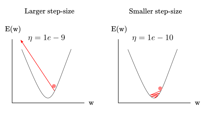
This is very strange. What is going on? In simple terms, the step-size is so large that after the first iteration, the error is so far-off from the minima of the function, that it can’t find its way in the right direction after that. Instead, the error starts to spiral out of control until it blows up and your computer runs out of memory. Remember, the ADALINE computes the $\hat{y}$ by multiplying each feature by the weights. Consider a bird with $x_1 = 10,000$ and $x_2 = 300$. Let’s compute the predicted value for that case:

$\hat{y} = 10,000*0.01 + 0.01*300 + 0.01*1 = 103.01$

Considering that now the error is computed as:

$error = (1 - 103.01)^2 = 10,406$

That’s a huge number. With enough data, the network should learn to reduce the $w_i$ until are small enough to make sensible predictions. But, if you start with predictions that are too far-off, the network may become unable to get back on track. Figure 7 succinctly illustrate this idea.

Figure 7

Linear separability constraint

We explored the linear separability constraint in detail in the perceptron Chapter, therefore we will explore this more briefly here. Let’s generate a new dataset, with Albatross and Condors.

condor_weight_mean = 12000 # in grams
condor_weight_variance = 1000 # in grams
condor_wingspan_mean = 290 # in cm
condor_wingspan_variance = 15 # in cm 
n_samples = 100
target = -1
seed = 100

# cX: feature matrix (weight, wingspan)
# cy: target value (1)
cX, cy = species_generator(condor_weight_mean, condor_weight_variance,
                           condor_wingspan_mean, condor_wingspan_variance,
                           n_samples,target,seed )

condor_dic = {'weight-(gm)': cX[:,0],
             'wingspan-(cm)': cX[:,1], 
             'species': cy,
             'url': "https://raw.githubusercontent.com/pabloinsente/nn-mod-cog/master/notebooks/images/condor.png"}

# put values in a relational table (pandas dataframe)
condor_df = pd.DataFrame(condor_dic)

df2 = albatross_df.append(condor_df, ignore_index=True)

alt.Chart(df2).mark_image(
    width=20,
    height=20
).encode(
    alt.X("weight-(gm)", scale=alt.Scale(domain=(6000, 16000))),
    alt.Y("wingspan-(cm)", scale=alt.Scale(domain=(220, 360))),
    url="url"
).properties(
title="Chart 3"
)

From Chart 3 is clear that there is no way to trace a line to separate albatross from condors based on the available features. Let’s train the ADALINE to test performance on this dataset.

df_shuffle2 = df2.sample(frac=1, random_state=1).reset_index(drop=True)
X = df_shuffle2[['weight-(gm)','wingspan-(cm)']].to_numpy()
y = df_shuffle2['species'].to_numpy()

w_3, mse_3 = fit(X, y, eta=1e-10, n_iter=12)

y_pred = predict(X,w_3)
num_correct_predictions = (y_pred == y).sum()
accuracy = (num_correct_predictions / y.shape[0]) * 100
print('Perceptron accuracy: %.2f%%' % accuracy)

Perceptron accuracy: 50.00%

mse_df["mse_3"] = mse_3
alt.Chart(mse_df).mark_line().encode(
    x="time-step", y="mse_3"
).properties(
    title='Chart 4'
)

The ADALINE accuracy drops to 50%, basically random guessing, given the same $\eta$ and iterations, but different a dataset (a nonlinearly separable one). You would be able to obtain better accuracy by a combination of tweaking $\eta$ and iterations, but it would never reach zero. Yet, it illustrates the fact that now the problem became really hard for the network. Finally, Chart 4 shows how baffling is the MSE over iterations with these parameters.

ADALINE limitations summary

Summarizing, the ADALINE :

is vulnerable to error/gradient explosion if an inappropriate learning rate has been chosen.
it can’t overcome the linear separability problem. It is a linear model, still.

Conclusions

With the ADALINE, Widrow and Hoff introduced for the first time the application of learning via gradient descent in the context of neural network models. If you are familiar with the contemporary literature in neural networks, you may be thinking I’m wrong or even lying. “Everybody knows that Rumelhart, Hinton, and Williams were the first ones on doing this in 1985”. What Rumelhart, Hinton, and Williams introduced, was a generalization of the gradient descend method, the so-called “backpropagation” algorithm, in the context of training multi-layer neural networks with non-linear processing units. Hence, it wasn’t actually the first gradient descent strategy ever applied, just the more general.

We saw in practice how training a neural network with the Widrow and Hoff approach dramatically reduced the training time compared to the perceptron learning procedure.

Although the ADALINE had a great impact in areas like telecommunications and engineering, its influence in the cognitive science community was very limited. Nonetheless, the methodological innovation introduced by Widrow and Hoff meant a step forward in what today we know is standard algorithms to train neural networks.

References

Talbert, L. R., Groner, G. F., & Koford, J. S. (1963). Real-Time Adaptive Speech-Recognition System. The Journal of the Acoustical Society of America, 35(5), 807–807.
Widrow, B., & Hoff, M. E. (1960). Adaptive switching circuits (No. TR-1553-1). Stanford Univ Ca Stanford Electronics Labs.
Widrow, B., & Lehr, M. A. (1990). 30 years of adaptive neural networks: perceptron, madaline, and backpropagation. Proceedings of the IEEE, 78(9), 1415-1442.
Widrow, B., & Lehr, M. A. (1995). Perceptrons, Adalines, and backpropagation. The handbook of brain theory and neural networks, 719-724.

catbug88@home:~$

Archive

About