The Multilayer Perceptron - Theory and Implementation of the Backpropagation Algorithm

20 Mar 2020

Share this:

Learning objectives

Understand the principles behind the creation of the multilayer perceptron
Identify how the multilayer perceptron overcame many of the limitations of previous models
Expand understanding of learning via gradient descent methods
Develop a basic code implementation of the multilayer perceptron in Python
Be aware of the main limitations of multilayer perceptrons

Historical and theoretical background

The origin of the backpropagation algorithm

Neural networks research came close to become an anecdote in the history of cognitive science during the ’70s. The majority of researchers in cognitive science and artificial intelligence thought that neural nets were a silly idea, they could not possibly work. Minsky and Papert even provided formal proofs about it 1969. Yet, as any person that has been around science long enough knows, there are plenty of stubborn researchers that will continue paddling against the current in pursue of their own ideas.

David Rumelhart first heard about perceptrons and neural nets in 1963 while in graduate school at Stanford. At the time, he was doing research in mathematical psychology, which although it has lots of equations, is a different field, so he did not pay too much attention to neural nets. It wasn’t until the early ’70s that Rumelhart took neural nets more seriously. He was in pursuit of a more general framework to understand cognition. Mathematical psychology looked too much like a disconnected mosaic of ad-doc formulas for him. By the late ’70s, Rumelhart was working at UC San Diego. He and some colleagues formed a study group about neural networks in cognitive science, that eventually evolved into what is known as the “Parallel Distributed Processing” (PDP) research group. Among the members of that group were Geoffrey Hinton, Terrence Sejnowski, Michael I. Jordan, Jeffrey L. Elman, and others that eventually became prominent researchers in the neural networks and artificial intelligence fields.

The original intention of the PDP group was to create a compendium of the most important research on neural networks. Their enterprise eventually evolved into something larger, producing the famous two volumes book where the so-called “backpropagation” algorithm was introduced, along with other important models and ideas. Although most people today associate the invention of the gradient descent algorithm with Hinton, the person that came up the idea was David Rumelhart, and as in most things in science, it was just a small change to a previous idea. Rumelhart and James McClelland (another young professor at UC San Diego at the time) wanted to train a neural network with multiple layers and sigmoidal units instead of threshold units (as in the perceptron) or linear units (as in the ADALINE), but they did not how to train such a model. Rumelhart knew that you could use gradient descent to train networks with linear units, as Widrow and Hoff did, so he thought that he might as well pretend that sigmoids units were linear units and see what happens. It worked, but he realized that training the model took too many iterations, so the got discouraged and let the idea aside for a while.

Backpropagation remained dormant for a couple of years until Hinton picked it up again. Rumelhart introduced the idea to Hinton, and Hinton thought it was a terrible idea. I could not work. He knew that backpropagation could not break the symmetry between weights and it will get stuck in local minima. He was passionate about energy-based systems known as Boltzmann machines, which seemed to have nicer mathematical properties. Yet, as he failed to solve more and more problems with Boltzmann machines he decided to try out backpropagation, mostly out of frustration. It worked amazingly well, way better than Boltzmann machines. He got in touch with Rumelhart about their results and both decided to include a backpropagation chapter in the PDP book and published Nature paper along with Ronald Williams. The Nature paper became highly visible and the interest in neural networks got reignited for at least the next decade. And that is how backpropagation was introduced: by a mathematical psychologist with no training in neural nets modeling and a neural net researcher that thought it was a terrible idea.

Overcoming limitations and creating advantages

Truth be told, “multilayer perceptron” is a terrible name for what Rumelhart, Hinton, and Williams introduced in the mid-‘80s. It is a bad name because its most fundamental piece, the training algorithm, is completely different from the one in the perceptron. Therefore, a multilayer perceptron it is not simply “a perceptron with multiple layers” as the name suggests. True, it is a network composed of multiple neuron-like processing units but not every neuron-like processing unit is a perceptron. If you were to put together a bunch of Rossenblat’s perceptron in sequence, you would obtain something very different from what most people today would call a multilayer perceptron. If anything, the multi-layer perceptron is more similar to the Widrow and Hoff ADALINE, and in fact, Widrow and Hoff did try multi-layer ADALINEs, known as MADALINEs (i.e., many ADALINEs), but they did not incorporate non-linear functions.

Now, the main reason for the resurgence of interest in neural networks was that finally someone designed an architecture that could overcome the perceptron and ADALINE limitations: to solve problems requiring non-linear solutions. Problems like the famous XOR (exclusive or) function (to learn more about it, see the “Limitations” section in the “The Perceptron” and “The ADALINE” blogposts).

Further, a side effect of the capacity to use multiple layers of non-linear units is that neural networks can form complex internal representations of entities. The perceptron and ADALINE did not have this capacity. They both are linear models, therefore, it doesn’t matter how many layers of processing units you concatenate together, the representation learned by the network will be a linear model. You may as well dropped all the extra layers and the network eventually would learn the same solution that with multiple layers (see Why adding multiple layers of processing units does not work for an explanation). This capacity is important in so far complex multi-level representation of phenomena is -probably- what the human mind does when solving problems in language, perception, learning, etc.

Finally, the backpropagation algorithm effectively automates the so-called “feature engineering” process. If you have ever done data analysis of any kind, you may have come across variables or features that were not in the original data but was created by transforming or combining other variables. For instance, you may have variables for income and education, and combine those to create a socio-economic status variable. That variable may have a predictive capacity above and beyond income and education in isolation. With a multilayer neural network with non-linear units trained with backpropagatio such a transformation process happens automatically in the intermediate or “hidden” layers of the network. Those intermediate representations often are hard or impossible to interpret for humans. They may make no sense whatsoever for us but somehow help to solve the pattern recognition problem at hand, so the network will learn that representation. Does this mean that neural nets learn different representations from the human brain? Maybe, maybe not. The problem is that we don’t have direct access to the kind of representations learned by the brain either, and a neural net will seldom be trained with the same data that a human brain is trained in real life.

The application of the backpropagation algorithm in multilayer neural network architectures was a major breakthrough in the artificial intelligence and cognitive science community, that catalyzed a new generation of research in cognitive science. Nonetheless, it took several decades of advance on computing and data availability before artificial neural networks became the dominant paradigm in the research landscape as it is today. Next, we will explore its mathematical formalization and application.

Mathematical formalization

The classical multilayer perceptron as introduced by Rumelhart, Hinton, and Williams, can be described by:

a linear function that aggregates the input values
a sigmoid function, also called activation function
a threshold function for classification process, and an identity function for regression problems
a loss or cost function that computes the overall error of the network
a learning procedure to adjust the weights of the network, i.e., the so-called backpropagation algorithm

Linear function

The linear aggregation function is the same as in the perceptron and the ADALINE. But, with a couple of differences that change the notation: now we are dealing multiple layers and processing units. The conventional way to represent this is with linear algebra notation. This is not a course of linear algebra, reason I won’t cover the mathematics in detail. However, I’ll introduce enough concepts and notation to understand the fundamental operations involved in the neural network calculation. The most important aspect is to understand what is a matrix, a vector, and how to multiply them together.

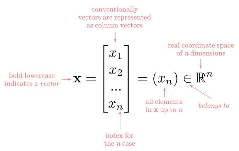
A vector is a collection of ordered numbers or scalars. If you are familiar with data analysis, a vector is like a column or row in a dataframe. If you are familiar with programming, a vector is like an array or a list. A generic Vector $\bf{x}$ is defined as:

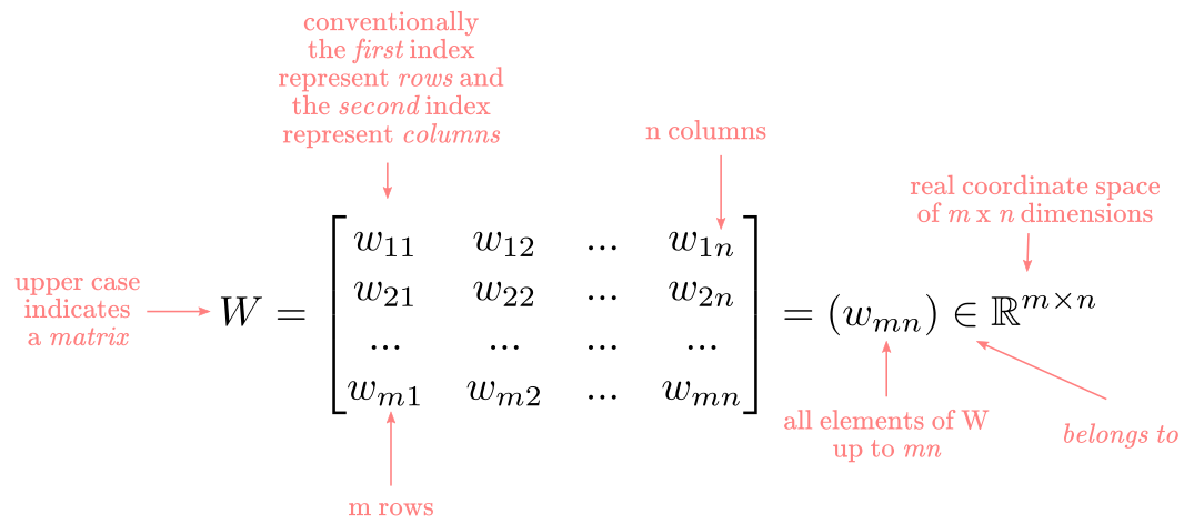
A matrix is a collection of vectors or lists of numbers. In data analysis, this is equivalent to a 2-dimensional dataframe. In programming is equivalent to a multidimensional array or a list of lists. A generic matrix $W$ is defined as:

Using this notation, let’s look at a simplified example of a network with:

3 inputs units
1 hidden layer with 2 units

Like the one in Figure 1

Figure 1

The input vector for our first training example would look like:

$\bf{x=} \begin{bmatrix} x_1 \\ x_2 \\ x_3 \\ \end{bmatrix}$

Since we have 3 input units connecting to hidden 2 units we have 3x2 weights. This is represented with a matrix as:

$W= \begin{bmatrix} w_{11} & w_{12}\\ w_{21} & w_{22}\\ w_{31} & w_{32} \end{bmatrix}$

The output of the linear function equals to the multiplication of the vector $\bf{x}$ and the matrix $W$. To perform the multiplication in this case we need to transpose the matrix $W$ to match the number of columns in $W$ with the number of rows in $\bf{x}$. Transposing means to “flip” the columns of $W$ such that the first column becomes the first row, the second column becomes the second row, and so forth. The matrix-vector multiplication equals to:

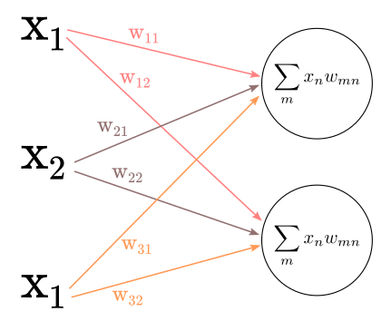
${\bf z=} W^T\times {\bf x=} \begin{bmatrix} w_{11} & w_{12} & w_{13} \\ w_{21} & w_{22} & w_{23} \\ \end{bmatrix} \begin{bmatrix} x_1 \\ x_2 \\ x_3 \\ \end{bmatrix}$ ${\bf z=} W^T\times {\bf x=} \begin{bmatrix} x_1w_{11} + x_2w_{12} + x_3w_{13}\\ x_1w_{21} + x_2w_{22} + x_3w_{23} \end{bmatrix} = \begin{bmatrix} z_1 \\ z_2 \end{bmatrix}$

The previous matrix operation in summation notation equals to:

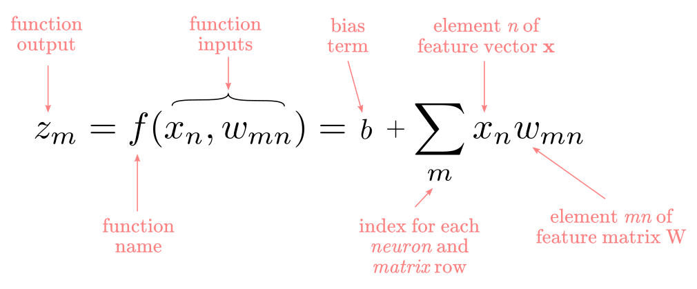
Here, $f$ is a function of each element of the vector $\bf{x}$ and each element of the matrix $W$. The $m$ index identifies the rows in $W^T$ and the rows in $\bf{z}$. The $n$ index indicates the columns in $W^T$ and the rows in $\bf{x}$. Notice that we add a $b$ bias term, that has the role to simplify learning a proper threshold for the function. If you are curious about that read the “Linear aggregation function” section here. In sum, the linear function is a weighted sum of the inputs plus a bias.

Sigmoid function

Each element of the $\bf{z}$ vector becomes an input for the sigmoid function $\sigma$():

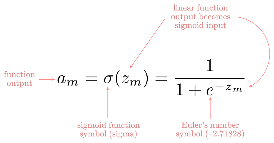
The output of $\sigma(z_m)$ is another $m$ dimensional vector $a$, one entry for each unit in the hidden layer like:

$\bf{a}= \begin{bmatrix} a_1 \\ a_2 \end{bmatrix}$

Here, $a$ stands for “activation”, which is a common way to refer to the output of hidden units. This sigmoid function “wrapping” the outcome of the linear function is commonly called activation function. The idea is that a unit gets “activated” in more or less the same manner that a neuron gets activated when a sufficiently strong input is received. The selection of a sigmoid is arbitrary. Many different non-linear functions could be selected at this stage in the network, like a Tanh or a ReLU. Unfortunately, there is no principled way to chose activation functions for hidden layers. It is mostly a matter of trial and error.

A nice property of sigmoid functions is they are “mostly linear” but they saturate as they approach 1 and 0 in the extremes. Chart 1 shows the shape of a sigmoid function (blue line) and the point where the gradient is at its maximum (the red line connecting the blue line).

from scipy.special import expit
import numpy as np
import altair as alt
import pandas as pd
z = np.arange(-5.0,5.0, 0.1)
a = expit(z)
df = pd.DataFrame({"a":a, "z":z})
df["z1"] = 0
df["a1"] = 0.5
sigmoid = alt.Chart(df).mark_line().encode(x="z", y="a")
threshold = alt.Chart(df).mark_rule(color="red").encode(x="z1", y="a1")
(sigmoid + threshold).properties(title='Chart 1')

Output function

For binary classification problems each output unit implements a threshold function as:

$\hat{y} = f(a_m) \begin{cases} +1, & \text{if } a \text{ > 0.5} \\ -1, & \text{otherwise} \end{cases}$

For regression problems (problems that require a real-valued output value like predicting income or test-scores) each output unit implements an identity function as:

$\hat{y}=f(a_m)=a_m$

In simple terms, an identity function returns the same value as the input. It does nothing. The point is that the $a$ is already the output of a linear function, therefore, it is the value that we need for this kind of problem.

For multiclass classification problems, we can use a softmax function as:

$\hat{y} = \sigma(a)_i = \frac{e^{\beta a_i}}{\sum_{j=1}^{k}e^{\beta z_j}}$

Cost function

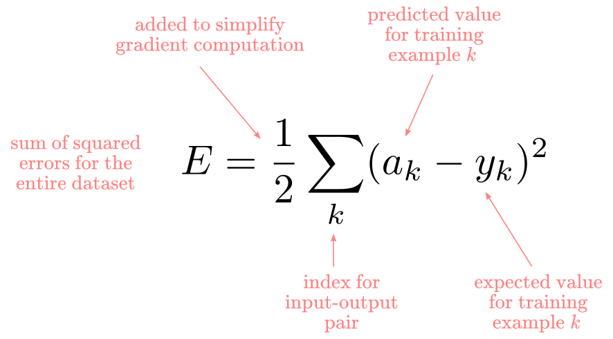
The cost function is the measure of “goodness” or “badness” (depending on how you like to see things) of the network performance. This can be a confusing term. People sometimes call it objective function, loss function, or error function. Conventionally, loss function usually refers to the measure of error for a single training case, cost function to the aggregate error for the entire dataset, and objective function is a more generic term referring to any measure of the overall error in a network. For instance, “mean squared error”, “sum of squared error”, and “binary cross-entropy” are all objective functions. For our purposes, I’ll use all those terms interchangeably: they all refer to the measure of performance of the network.

Nowadays, you would probably want to use different cost functions for different types of problems. In their original work, Rumelhart, Hinton, and Williams used the sum of squared errors defined as:

Forward propagation

All neural networks can be divided into two parts: a forward propagation phase, where the information “flows” forward to compute predictions and the error; and the backward propagation phase, where the backpropagation algorithm computes the error derivatives and update the network weights. Figure 2 illustrate a network with 2 input units, 3 hidden units, and 1 output unit.

Figure 2

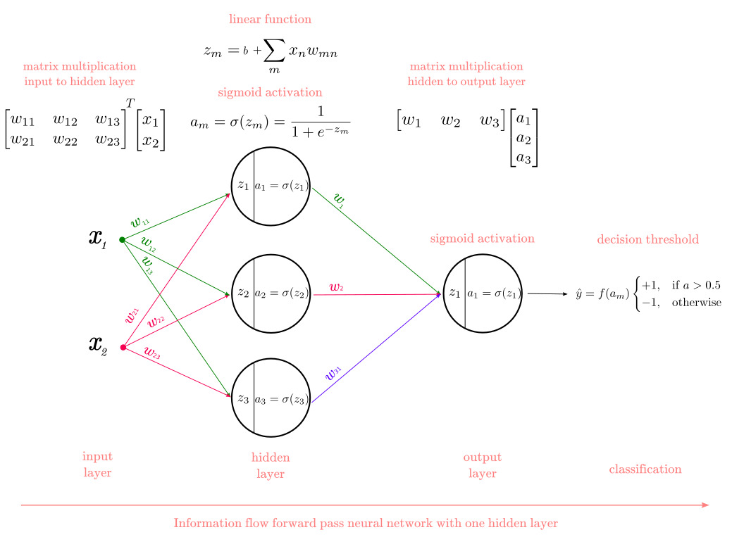
The forward propagation phase involves “chaining” all the steps we defined so far: the linear function, the sigmoid function, and the threshold function. Consider the network in Figure 2. Let’s label the linear function as $\lambda()$, the sigmoid function as $\sigma()$, and the threshold function as $\tau()$. Now, the network in Figure 2 can be represented as:

$\hat{y} = \tau(\sigma^{(2)}(\lambda^{(2)}(\sigma^{(1)}(\lambda^{(1)}(x_n, w_{mn})))))$

All neural networks can be represented as a composition of functions where each step is nested in the next step. For instance, we can add an extra hidden layer to the network in Figure 2 by:

$\hat{y} = \tau(\sigma^{(3)}(\lambda^{(3)}(\sigma^{(2)}(\lambda^{(2)}(\sigma^{(1)}(\lambda^{(1)}(x_n, w_{mn})))))))$

Backpropagation algorithm

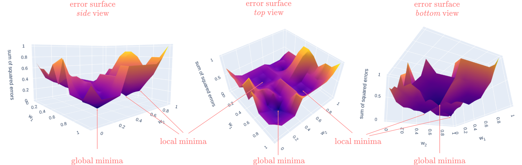
In the ADALINE blogpost I introduced the ideas of searching for a set of weights that minimize the error via gradient descent, and the difference between convex and non-convex optimization. If you have not read that section, I’ll encourage you to read that first. Otherwise, the important part is to remember that since we are introducing nonlinearities in the network the error surface of the multilayer perceptron is non-convex. This means that there are multiple “valleys” with “local minima”, along with the “global minima”, and that backpropagation is not guaranteed to find the global minima. Remember that the “global minima” is the point where the error (i.e., the value of the cost function) is at its minimum, whereas the “local minima” is the point of minimum error for a sub-section of the error surface. Figure 3 illustrates these concepts on a 3D surface. The vertical axis represents the error of the surface, and the other two axes represent different combinations of weights for the network. In the figure, you can observe how different combinations of weights produce different values of error.

Figure 3

Now we have all the ingredients to introduce the almighty backpropagation algorithm. Remember that our goal is to learn how the error changes as we change the weights of the network by tiny amount and that the cost function was defined as:

$E = \frac{1}{2}\sum_k(a_k - y_k)^2$

There is one piece of notation I’ll introduce to clarify where in the network are we at each step of the computation. I’ll use the superscript $L$ to index the outermost function in the network. For example, $a^{(L)}$ index the last sigmoid activation function at the output layer, $a^{(L-1)}$ index the previous sigmoid activation function at the hidden layer, and $x^{(L-2)}$ index the features in the input layer (which are the only thing in that layer). Think about this as moving from the right at $(L)$ to the left at $(L-2)$ in the computational graph of the network in Figure 4.

Backpropagation for single unit multilayer perceptron

In my experience, tracing the indices in backpropagation is the most confusing part, so I’ll ignore the summation symbol and drop the subscript $k$ to make the math as clear as possible. You can think of this as having a network with a single input unit, a single hidden unit, and a single output unit, as in Figure 4. We will first work out backpropagation for this simplified network and then expand for the multi-neuron case.

Figure 4

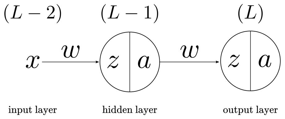
The whole purpose of backpropagation is to answer the following question: “How does the error change when we change the weights by a tiny amount?” (be aware that I’ll use the words “derivatives” and “gradients” interchangeably).

To accomplish this you have to realize the following:

The error $E$ depends on the value of the sigmoid activation function $a$.
The value of the sigmoid function activation function $a$ depends on the value of the linear function $z$.
The value of the linear function $z$ depends on the value of the weights $w$

Therefore, we can trace a change of dependence on the weights. This means we have to answer these three questions in a chain:

How does the error $E$ change when we change the activation $a$ by a tiny amount
How does the activation $a$ change when we change the activation $z$ by a tiny amount
How does $z$ change when we change the weights $w$ by a tiny amount

Such sequence can be mathematically expressed with the chain-rule of calculus as:

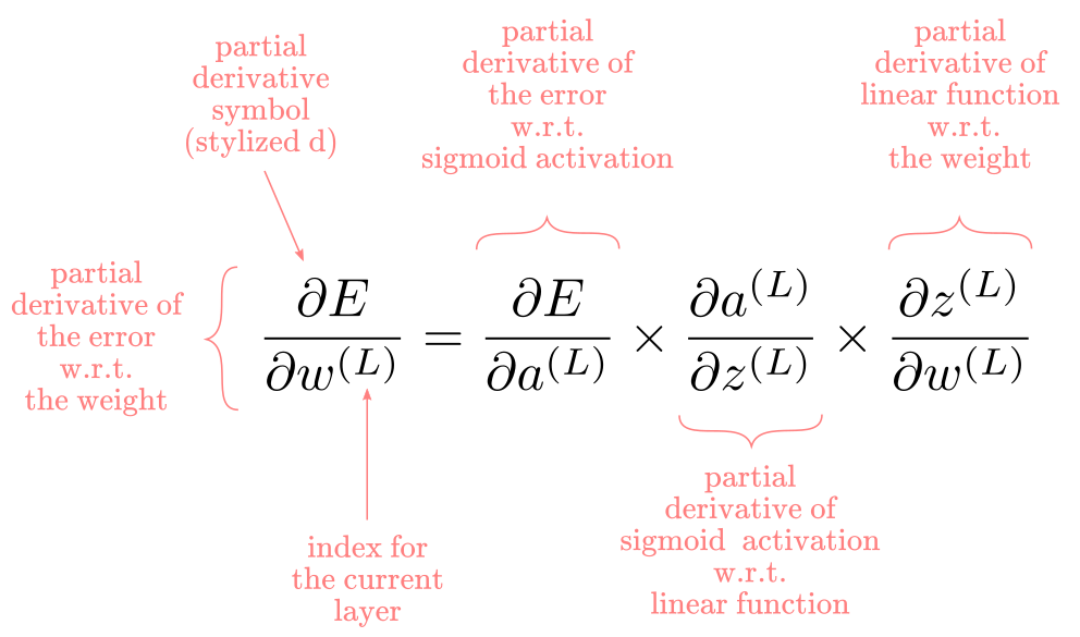
No deep knowledge of calculus is needed to understand the chain-rule. In essence, indicates how to differentiate composite functions, i.e., functions nested inside other functions. If you remember the section above this one, we showed that a multi-layer perceptron can be expressed as a composite function. Very convenient. The rule says that we take the derivative of the outermost function, and multiple by the derivative of the inside function, recursively. That’s it.

Good. Now, let’s differentiate each part of $\frac{\partial E}{\partial w^(L)}$. Let’s begin from the outermost part.

The derivative of the error with respect to (w.r.t) the sigmoid activation function is:

$\frac{\partial E}{\partial a^{(L)}} = a^{(L)} - y$

Next, the derivative of the sigmoid activation function w.r.t the linear function is:

$\frac{\partial a^{(L)}}{\partial z^{(L)}} = a^{(L)}(1-a^{(L)})$

Finally, the derivative of the linear function w.r.t the weights is:

$\frac{\partial z^{(L)}}{\partial w^{(L)}} = a^{(L-1)}$

If we put all the pieces together and replace we obtain:

$\frac{\partial E}{\partial w^{(L)}} = a^{(L)} - y \times a^{(L)}(1-a^{(L)}) \times a^{(L-1)}$

At this point, we have figured out how the error changes as we change the weight connecting the hidden layer and the output layer $w^{(L)}$. Amazing progress. We still need to know how the error changes as we adjust the weight connecting the input layer and the hidden layer $w^{(L-1)}$. Fortunately, this is pretty straightforward: we apply the chain-rule again, and again until we get there.

$\frac{\partial E}{\partial w^{(L-1)}} = \frac{\partial E}{\partial a^{(L)}} \times \frac{\partial a^{(L)}}{\partial z^{(L)}} \times \frac{\partial z^{(L)}}{\partial a^{(L-1)}} \times \frac{\partial a^{(L-1)}}{\partial z^{(L-1)}} \times \frac{\partial z^{(L-1)}}{\partial w^{(L-1)}}$

Again, replacing with the actual derivatives this becomes:

$\frac{\partial E}{\partial w^{(L-1)}} = a^{(L)} - y \times a^{(L)}(1-a^{(L)}) \times w^{(L)} \times a^{(L-1)}(1-a^{(L-1)}) \times x^{(L-1)}$

Fantastic. There is one tiny piece we haven’t mentioned: the derivative of the error with respect to the bias term $b$. There are two ways to approach this. One way is to treat the bias as another feature (usually with value 1) and add the corresponding weight to the matrix $W$. In such a case, the derivative of the weight for the bias is calculated along with the weights for the other features in the exact same manner. The other option is to compute the derivative separately as:

$\frac{\partial E}{\partial b^{(L)}} = \frac{\partial E}{\partial a^{(L)}} \times \frac{\partial a^{(L)}}{\partial z^{(L)}} \times \frac{\partial z^{(L)}}{\partial b^{(L)}}$

We already know the values for the first two derivatives. We just need to figure out the derivative for $\frac{\partial z^{(L)}}{\partial b^{(L)}}$. Now, remember that the slope of $z$ does not depend at all from $b$, because $b$ is just a constant value added at the end. Therefore, the derivative of the error w.r.t the bias reduces to:

$\frac{\partial E}{\partial b^{(L)}} = a^{(L)} - y \times a^{(L)}(1-a^{(L)})$

This is very convenient because it means we can reutilize part of the calculation for the derivative of the weights to compute the derivative of the biases.

The last missing part is the derivative of the error w.r.t. the bias $b$ in the $(L-1)$ layer:

$\frac{\partial E}{\partial b^{(L-1)}} = \frac{\partial E}{\partial a^{(L)}} \times \frac{\partial a^{(L)}}{\partial z^{(L)}} \times \frac{\partial z^{(L)}}{\partial a^{(L-1)}} \times \frac{\partial a^{(L-1)}}{\partial z^{(L-1)}} \times \frac{\partial z^{(L-1)}}{\partial b^{(L-1)}}$

Replacing with the actual derivatives for each expression:

$\frac{\partial E}{\partial b^{(L-1)}} = a^{(L)} - y \times a^{(L)}(1-a^{(L)}) \times w^{(L)} \times a^{(L-1)}(1-a^{(L-1)})$

Same as before, we can reuse part of the calculation for the derivative of $w^{(L-1)}$ to solve this. Every time we train a neural net wit backpropagation we will need to compute the derivatives for all the weight and biases as showed before.

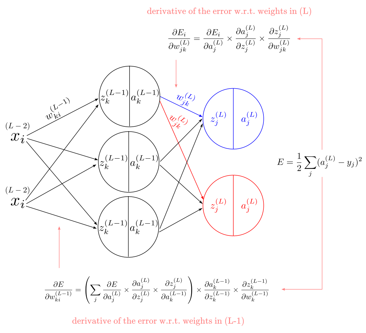
Backpropagation for multiple unit multilayer perceptron

Pretty much all neural networks you’ll find have more than one neuron. Until now, we have assumed a network with a single neuron per layer. The only difference between the expressions we have used so far and added more units is a couple of extra indices. For example, we can use the letter $j$ to index the units in the output layer, the letter $k$ to index the units in the hidden layer, and the letter $i$ to index the units in the input layer. We also need indices for the weights. For any network with multiple units, we will have more weights than units, which means we will need two subscripts to indicate each weight. This is visible in the weight matrix in Figure 2. We will index the weights as $w_{\text{destination-units} \text{, } \text{origin-units}}$. For instance, weights in $(L)$ become $w_{jk}$.

With all this notation in mind, our original equation for the derivative of the error w.r.t the weights in $(L)$ layer becomes:

$\frac{\partial E}{\partial w^{(L)}_{jk}} = \frac{\partial E_i}{\partial a^{(L)}_j} \times \frac{\partial a^{(L)}_j}{\partial z^{(L)}_j} \times \frac{\partial z^{(L)}_j}{\partial w^{(L)}_{jk}}$

Replacing with the derivatives:

$\frac{\partial E}{\partial w^{(L)}_{jk}} = a^{(L)}_j - y \times a^{(L)}_j(1-a^{(L)}_j) \times a^{(L-1)}_k$

There is a second thing to consider. This time we have to take into account that each sigmoid activation $a$ from $(L-1)$ layers impacts the error via multiple pathways (assuming a network with multiple output units). In Figure 5 this is illustrated by blue and red connections to the output layer. To reflect this, we add a summation symbol and the expression for the derivative of the error w.r.t the sigmoid activation becomes:

$\frac{\partial E}{\partial a^{(L-1)}_k} = \sum_{j} \frac{\partial E}{\partial a^{(L)}_j} \times \frac{\partial a^{(L)}_j}{\partial z^{(L)}_j} \times \frac{\partial z^{(L)}_j}{\partial a^{(L-1)}_k}$

Now, considering both the new subscripts and summation for $\frac{\partial E}{\partial a^{(L-1)}_k}$, we can apply the chain-rule one more time to compute the error derivatives for $w$ in $(L-1)$ as:

$\frac{\partial E}{\partial w^{(L-1)}_{ki}} = \left(\sum_{j} \frac{\partial E}{\partial a^{(L)}_j} \times \frac{\partial a^{(L)}_j}{\partial z^{(L)}_j} \times \frac{\partial z^{(L)}_j}{\partial a^{(L-1)}_k}\right) \times \frac{\partial a^{(L-1)}_k}{\partial z^{(L-1)}_k} \times \frac{\partial z^{(L-1)}_k}{\partial w^{(L-1)}_k}$

Replacing with the actual derivatives for each expression we obtain:

$\frac{\partial E}{\partial w^{(L-1)}_{ki}} = a^{(L)}_j - y \times a^{(L)}_j(1-a^{(L)}_j) \times w^{(L)}_{jk} \times a^{(L-1)}_k(1-a^{(L-1)}_k) \times x^{(L-1)}_i$

Considering the new indices, the derivative for the error w.r.t the bias $b$ becomes:

$\frac{\partial E}{\partial b_j^{(L)}} = \frac{\partial E}{\partial a^{(L)}_j} \times \frac{\partial a^{(L)}_j}{\partial z^{(L)}_j} \times \frac{\partial z^{(L)}_j}{\partial b^{(L)}_j}$

Replacing with the actual derivatives we get:

$\frac{\partial E}{\partial b^{(L)}_j} = a^{(L)}_j - y \times a^{(L)}_j(1-a^{(L)}_j)$

Last but not least, the expression for the bias $b$ at layer $(L-1)$ is:

$\frac{\partial E}{\partial b^{(L-1)}} = \frac{\partial E}{\partial a^{(L)}_j} \times \frac{\partial a^{(L)}_j}{\partial z^{(L)}_j} \times \frac{\partial z^{(L)}_j}{\partial a^{(L-1)}_k} \times \frac{\partial a^{(L-1)}_k}{\partial z^{(L-1)}_k} \times \frac{\partial z^{(L-1)}_k}{\partial b^{(L-1)}_k}$

Replacing with the actual derivatives we get:

$\frac{\partial E}{\partial b^{(L-1)}} = a^{(L)}_j - y \times a^{(L)}_j(1-a^{(L)}_j) \times w^{(L)}_{jk} \times a^{(L-1)}_k(1-a^{(L-1)}_k)$

And that’s it! Those are all the pieces for the backpropagation algorithm. Probably, the hardest part is to track all the indices. To further clarify the notation you can look at the diagram in Figure 5 that exemplifies where each piece of the equation is located.

Figure 5

Backpropagation weight update

We learned how to compute the gradients for all the weights and biases. Now we just need to use the computed gradients to update the weights and biases values. This is actually when the learning happens. We do this by taking a portion of the gradient and substracting that to the current weight and bias value.

For the wegiths $w_{jk}$ in the $(L)$ layer we update by:

$w_{jk}^{L} = w_{jk}^{L} - \eta \times \frac{\partial E}{\partial w_{jk}^{L}}$

For the wegiths $w_{ki}$ in the $(L-1)$ layer we update by:

$w_{ki}^{L-1} = w_{ki}^{L-1} - \eta \times \frac{\partial E}{\partial w_{ki}^{L-1}}$

For the bias $b$ in the $(L)$ layer we update by:

$b^{(L)} = b^{(L)} - \eta \times \frac{\partial E}{\partial b^{(L)}}$

For the bias $b$ in the $(L-1)$ layer we update by:

$b^{(L-1)} = b^{(L-1)} - \eta \times \frac{\partial E}{\partial b^{(L-1)}}$

Where $\eta$ is the step size or learning rate.

If you are not familiar with the idea of a learning rate, you can review the ADALINE blogpost where I briefly explain the concept. In brief, a learning rate controls how fast we descend over the error surface given the computed gradient. This is important because we want to give steps just large enough to reach the minima of the surface at any point we may be when searching for the weights. You can see a more deep explanation here.

I don’t know about you but I have to go over several rounds of carefully studying the equations behind backpropagation to finally understand them fully. This may or not be true for you, but I believe the effort pays off as backpropagation is the engine of every neural network model today. Regardless, the good news is the modern numerical computation libraries like NumPy, Tensorflow, and Pytorch provide all the necessary methods and abstractions to make the implementation of neural networks and backpropagation relatively easy.

Code implementation

We will implement a multilayer-perceptron with one hidden layer by translating all our equations into code. One important thing to consider is that we won’t implement all the loops that the summation notation implies. Loops are known for being highly inefficient computationally, so we want to avoid them. Fortunately, we can use matrix operations to achieve the exact same result. This means that all the computations will be “vectorized”. If you are not familiar with vectorization you just need to know that instead of looping over each row in our training dataset we compute the outcome for each row all at once using linear algebra operations. This makes computation in neural networks highly efficient compared to using loops. To do this, I’ll only use NumPy which is the most popular library for matrix operations and linear algebra in Python.

Remember that we need to computer the following operations in order:

linear function aggregation $z$
sigmoid function activation $a$
cost function (error) calculation $E$
derivative of the error w.r.t. the weights $w$ and bias $b$ in the $(L)$ layer
derivative of the error w.r.t. the weights $w$ and bias $b$ in the $(L-1)$ layer
weight and bias update for the $(L)$ layer
weight and bias update for the $(L-1)$ layer

Those operations over the entire dataset comprise a single “iteration” or “epoch”. Generally, we need to perform multiple repetitions of that sequence to train the weights. That loop can’t be avoided unfortunately and will be part of the “fit” function.

Initialize training parameters

import numpy as np

def init_parameters(n_features, n_neurons, n_output):
    """generate initial parameters sampled from an uniform distribution
    
    Args:
        n_features (int): number of feature vectors 
        n_neurons (int): number of neurons in hidden layer
        n_output (int): number of output neurons
    
    Returns:
        parameters dictionary:
            W1: weight matrix, shape = [n_features, n_neurons]
            b1: bias vector, shape = [1, n_neurons]
            W2: weight matrix, shape = [n_neurons, n_output]
            b2: bias vector, shape = [1, n_output]
    """
    
    np.random.seed(100) # for reproducibility
    W1 = np.random.uniform(size=(n_features,n_neurons))
    b1 = np.random.uniform(size=(1,n_neurons))
    W2 = np.random.uniform(size=(n_neurons,n_output))
    b2 = np.random.uniform(size=(1,n_output))
    
    parameters = {"W1": W1,
                  "b1": b1,
                  "W2": W2,
                  "b2": b2}
    
    return parameters

Backpropagation is very sensitive to the initialization of parameters. For instance, in the process of writing this tutorial I learned that this particular network has a hard time finding a solution if I sample the weights from a normal distribution with mean = 0 and standard deviation = 0.01, but it does much better sampling from a uniform distribution. In any case, it is common practice to initialize the values for the weights and biases to some small values.

Compute $z$: linear function

def linear_function(W, X, b):
    """computes net input as dot product
    
    Args:
        W (ndarray): weight matrix
        X (ndarray): matrix of features
        b (ndarray): vector of biases
        
    Returns:
        Z (ndarray): weighted sum of features
        """
    
    return (X @ W)+b

Compute $a$: sigmoid activation function

def sigmoid_function(Z):
    """computes sigmoid activation element wise
    
    Args:
        Z (ndarray): weighted sum of features
    
    Returns: 
        S (ndarray): neuron activation
    """
    
    return 1/(1+np.exp(-Z)) 

Compute cost (error) function $E$

def cost_function(A, y):
    """computes squared error
    
    Args:
        A (ndarray): neuron activation
        y (ndarray): vector of expected values
    
    Returns:
        E (float): total squared error"""
    
    return (np.mean(np.power(A - y,2)))/2

Compute predictions $\hat{y}$ with learned parameters

def predict(X, W1, W2, b1, b2):
    """computes predictions with learned parameters
    
    Args:
        X (ndarray): matrix of features
        W1 (ndarray): weight matrix for the first layer
        W2 (ndarray): weight matrix for the second layer
        b1 (ndarray): bias vector for the first layer
        b2 (ndarray): bias vector for the second layer
        
    Returns:
        d (ndarray): vector of predicted values
    """
    
    Z1 = linear_function(W1, X, b1)
    S1 = sigmoid_function(Z1)
    Z2 = linear_function(W2, S1, b2)
    S2 = sigmoid_function(Z2)
    return np.where(S2 >= 0.5, 1, 0)

Since I plan to solve a binary classification problem, we define a threshold function that takes the output of the last sigmoid activation function and returns a 0 or a 1 for each class.

Backpropagation and training loop

def fit(X, y, n_features=2, n_neurons=3, n_output=1, iterations=10, eta=0.001):
    """Multi-layer perceptron trained with backpropagation
    
    Args:
        X (ndarray): matrix of features
        y (ndarray): vector of expected values
        n_features (int): number of feature vectors 
        n_neurons (int): number of neurons in hidden layer
        n_output (int): number of output neurons
        iterations (int): number of iterations over the training set
        eta (float): learning rate
        
    Returns: 
        errors (list): list of errors over iterations
        param (dic): dictionary of learned parameters
    """
    
    ## ~~ Initialize parameters ~~##
    param = init_parameters(n_features=n_features, 
                            n_neurons=n_neurons, 
                            n_output=n_output)

    ## ~~ storage errors after each iteration ~~##
    errors = []
    
    for _ in range(iterations):
        
        ##~~ Forward-propagation ~~##
        
        Z1 = linear_function(param['W1'], X, param['b1'])
        S1 = sigmoid_function(Z1)
        Z2 = linear_function(param['W2'], S1, param['b2'])
        S2 = sigmoid_function(Z2)
        
        ##~~ Error computation ~~##
        error = cost_function(S2, y)
        errors.append(error)
        
        ##~~ Backpropagation ~~##
        
        # update output weights
        delta2 = (S2 - y)* S2*(1-S2)
        W2_gradients = S1.T @ delta2
        param["W2"] = param["W2"] - W2_gradients * eta

        # update output bias
        param["b2"] = param["b2"] - np.sum(delta2, axis=0, keepdims=True) * eta

        # update hidden weights
        delta1 = (delta2 @ param["W2"].T )* S1*(1-S1)
        W1_gradients = X.T @ delta1 
        param["W1"] = param["W1"] - W1_gradients * eta

        # update hidden bias
        param["b1"] = param["b1"] - np.sum(delta1, axis=0, keepdims=True) * eta
        
    return errors, param

Here is where we put everything together to train the network. The first part of the function initializes the parameters by calling the init_parameters function. The loop (for _ in range(iterations)) in the second part of the function is where all the action happens:

the Forward-propagation section chains the linear and sigmoid functions to compute the network output.
the Error computation section computes the cost function value after each iteration.
the Backpropagation section does two things:
- computes the gradients for the weights and biases in the $(L)$ and $(L-1)$ layers
- update the weights and biases in the $(L)$ and $(L-1)$ layers
the fit function returns a list of the errors after each iteration and an updated dictionary with the learned weights and biases.

Application: solving the XOR problem

If you have read this and the previous blogpost in this series, you should know by now that one of the problems that brought about the “demise” of the interest in neural network models was the infamous XOR (exclusive or) problem. This was just one example of a large class of problems that can’t be solved with linear models as the perceptron and ADALINE. As an act of redemption for neural networks from this criticism, we will solve the XOR problem using our implementation of the multilayer-perceptron.

Generate features and target

The first is to generate the targets and features for the XOR problem. Table 1 shows the matrix of values we need to generate, where $x_1$ and $x_2$ are the features and $y$ the expected output.

Table 1: Truth Table For XOR Function

$x_1$	$x_2$	$y$
0	0	0
0	1	1
1	0	1
1	1	0

# expected values
y = np.array([[0, 1, 1, 0]]).T

# features
X = np.array([[0, 0, 1, 1],
              [0, 1, 0, 1]]).T

Multilayer perceptron training

We will train the network by running 5,000 iterations with a learning rate of $\eta = 0.1$.

errors, param = fit(X, y, iterations=5000, eta=0.1)

Multilayer perceptron predictions and error

y_pred = predict(X, param["W1"], param["W2"], param["b1"], param["b2"])
num_correct_predictions = (y_pred == y).sum()
accuracy = (num_correct_predictions / y.shape[0]) * 100
print('Multi-layer perceptron accuracy: %.2f%%' % accuracy)

Multi-layer perceptron accuracy: 100.00%

import altair as alt
import pandas as pd
alt.data_transformers.disable_max_rows()

df = pd.DataFrame({"errors":errors, "time-step": np.arange(0, len(errors))})

alt.Chart(df).mark_line().encode(x="time-step", y="errors").properties(title='Chart 2')

The error curve is revealing. After the first few iterations the error dropped fast to around 0.13, and from there went down more gradually. If you are wondering how the accuracy is 100% although the error is not zero, remember that the binary predictions have no business in the error computation and that many different sets of weights may generate the correct predictions.

Application: multilayer perceptron with Keras

The reason we implemented our own multilayer perceptron was for pedagogical purposes. Richard Feynman once famously said: “What I cannot create I do not understand”, which is probably an exaggeration but I personally agree with the principle of “learning by creating”. Learning to build neural networks is similar to learn math (maybe because they are literally math): yes, you’ll end up using a calculator to compute almost everything, yet, we still do the exercise of computing systems of equations by hand when learning algebra. There is a deeper level of understanding that is unlocked when you actually get to build something from scratch.

Nonetheless, there is no need to go through this process every time. Nowadays, we have access to very good libraries to build neural networks. Keras is a popular Python library for this. Keras main strength is the simplicity and elegance of its interface (sometimes people call it “API”). Keras hides most of the computations to the users and provides a way to define neural networks that match with what you would normally do when drawing a diagram. There are many other libraries you may hear about (Tensorflow, PyTorch, MXNet, Caffe, etc.) but I’ll use this one because is the best for beginners in my opinion.

Next, we will build another multi-layer perceptron to solve the same XOR Problem and to illustrate how simple is the process with Keras.

This time, I’ll put together a network with the following characteristics:

Input layer with 2 neurons (i.e., the two features).
One hidden layer with 16 neurons with sigmoid activation functions.
Output layer with 1 neuron with a sigmoid activation (i.e., a target value of 0 or 1).
Mean squared error as the cost (or loss) function.
“Adam” optimizer. This a variation of gradient descent that (sometimes) speed up the process by adapting the learning rate for each parameter in the network. It has the advantage that we don’t need to manually search for the learning rate.

import numpy as np
from keras.models import Sequential
from keras.layers.core import Dense

Using TensorFlow backend.

Let’s generate the training data

# expected values
y = np.array([[0, 1, 1, 0]]).T

# features
X = np.array([[0, 0, 1, 1],
              [0, 1, 0, 1]]).T

Let’s examine the model definition:

Sequential() specifies that the network is a linear stack of layers
model.add() adds the hidden layer.
Dense means that neurons between layers are fully connected
input_dim defines the number of features in the training dataset
activation defines the activation function
loss selects the cost function
optimizer selects the learning algorithm
metrics selects the performance metrics to be saved for further analysis
model.fit() initialize the training

model = Sequential()
model.add(Dense(16, input_dim=2, activation='sigmoid'))
model.add(Dense(1, activation='sigmoid'))

model.compile(loss='mean_squared_error',
              optimizer='adam',
              metrics=['binary_accuracy', 'mean_squared_error'])

history = model.fit(X, y, epochs=3000, verbose=0)

errors = history.history['loss']

df2 = pd.DataFrame({"errors":errors, "time-step": np.arange(0, len(errors))})

alt.Chart(df2).mark_line().encode(x="time-step", y="errors").properties(title='Chart 3')

The main difference between the error curve for our own implementation (Chart 2) and the Keras version is the speed at which the error declines. This is mostly accounted for the selection of the Adam optimizer instead of “plain” backpropagation.

y_pred = model.predict(X).round()
num_correct_predictions = (y_pred == y).sum()
accuracy = (num_correct_predictions / y.shape[0]) * 100
print('Multi-layer perceptron accuracy: %.2f%%' % accuracy)

Multi-layer perceptron accuracy: 100.00%

Again, we reached 100% of accuracy.

Multilayer perceptron limitations

Multilayer perceptrons (and multilayer neural networks more) generally have many limitations worth mentioning. I will focus on a few that are more evident at this point and I’ll introduce more complex issues in later blogposts.

Training time

The first and more obvious limitation of the multilayer perceptron is training time. It takes an awful lot of iterations for the algorithm to learn to solve a very simple logic problem like the XOR. This is not an exception but the norm. Most neural networks you’d encounter in the wild nowadays need from hundreds up to thousands of iterations to reach their top-level accuracy. This has been a common point of criticism, particularly because human learning seems to be way more sample efficient.

There are multiple answers to the training time problem. A first argument has to do with raw processing capacity. It is seemingly obvious that a neural network with 1 hidden layer and 3 units does not get even close to the massive computational capacity of the human brain. Even if you consider a small subsection of the brain, and design a very large neural network with dozens of layers and units, the brain still has the advantage in most cases. Of course, this alone probably does not account for the entire gap between humans and neural networks but is a point to consider. A second argument refers to the massive past training experience accumulated by humans. Neural networks start from scratch every single time. Humans do not reset their storage memories and skills before attempting to learn something new. On the contrary, humans learn and reuse past learning experience across domains continuously. A third argument is related to the richness of the training data experienced by humans. Humans not only rely on past learning experiences but also on more complex and multidimensional training data. Humans integrate signals from all senses (visual, auditory, tactile, etc.) when learning which most likely speeds up the process. In any case, this is still a major issue and a hot topic of research.

Multilayer perceptrons are “fragile”

A second notorious limitation is how brittle multilayer perceptrons are to architectural decisions. An extra layer, a +0.001 in the learning rate, random uniform weight instead for random normal weights, and or even a different random seed can turn perfectly a functional neural network into a useless one. This is partially related to the fact we are trying to solve a nonconvex optimization problem. Gradient descent has no way to find the actual global minima in the error surface. You just can hope it will find a good enough local minima for your problem. All of this force neural network researchers to search over enormous combinatorial spaces of “hyperparameters” (i.e., like the learning rate, number layers, etc. Anything but the network weights and biases). In a way, you have to embrace the fact that perfect solutions are rarely found unless you are dealing with simple problems with known solutions like the XOR. Surprisingly, it is often the case that well designed neural networks are able to learn “good enough” solutions for a wide variety of problems. Creating more robust neural networks architectures is another present challenge and hot research topic.

The biological plasubility of backpropagation

The last issue I’ll mention is the elephant in the room: it is not clear that the brain learns via backpropagation. Rumelhart, Hinton, and Williams presented no evidence in favor of this assumption. You may think that it does not matter because neural networks do not pretend to be exact replicas of the brain anyways. Yet, it is a highly critical issue coming from the perspective of creating “biologically plausible” models of cognition, which is the PDP group perspective. Remember that one of the main problems for Rumelhart was to find a learning mechanism for networks with non-linear units. If the learning mechanism is not plausible, Does the model have any credibility at all? Fortunately, in the last 35 years we have learned quite a lot about the brain, and several researchers have proposed how the brain could implement “something like” backpropagation. Still, keep in mind that this is a highly debated topic and it may pass some time before we reach a resolution.

Conclusions

The introduction of multilayer perceptrons trained with backpropagation was a major breakthrough in cognitive science and artificial intelligence in the ’80s. It brought back to life a line of research that many thought dead for a while. The key for its success was its ability to overcome one of the major criticism from the previous decade: its inability to solve problems that required non-linear solutions.

From a cognitive science perspective, the real question is whether such advance says something meaningful about the plausibility of neural networks as models of cognition. That is a tough question. If you are in the “neural network team” of course you’d think it does. If you are more skeptic you’d rapidly point out to the many weaknesses and unrealistic assumptions on which neural networks depend on.

Maybe the best way of thinking about this type of advances in neural networks models of cognition is as another piece of a very complicated puzzle. The “puzzle” here is a working hypothesis: you are committed to the idea that the puzzle of cognition looks like a neural network when assembled, and your mission is to figure out all the pieces and putting them together. You may be wrong, maybe the puzzle at the end looks like something different, and you’ll be proven wrong. Yet, at least in this sense, multilayer perceptrons were a crucial step forward in the neural network research agenda.

References

Goodfellow, I., Bengio, Y., & Courville, A. (2016). Deep Feedforward Networks. In Deep Learning. MIT Press. https://www.deeplearningbook.org/contents/mlp.html

Kelley, H. J. (1960). Gradient theory of optimal flight paths. Ars Journal, 30(10), 947–954.

Bryson, A. E. (1961). A gradient method for optimizing multi-stage allocation processes. Proc. Harvard Univ. Symposium on Digital Computers and Their Applications, 72.

Rumelhart, D. E., Hinton, G. E., & Williams, R. J. (1986). Learning Internal Representations by Error Propagation. In Parallel Distributed Processing: Explorations in the Microestructure of Cognition (Vol. 1). MIT Press.

Rumelhart, D. E., Hinton, G. E., & Williams, R. J. (1986). Learning representations by back-propagating errors. Nature, 323(6088), 533–536.

Werbos, P. J. (1994). The roots of backpropagation: From ordered derivatives to neural networks and political forecasting (Vol. 1). John Wiley & Sons.

Useful on-line resources:

The internet is flooded with learning resourced about neural networks. Here a selection of my personal favorites for this topic:

catbug88@home:~$

Archive

About