The Recurrent Neural Network - Theory and Implementation of the Elman Network and LSTM

16 Apr 2020

Share this:

Learning objectives

Understand the principles behind the creation of the recurrent neural network
Obtain intuition about difficulties training RNNs, namely: vanishing/exploding gradients and long-term dependencies
Obtain intuition about mechanics of backpropagation through time BPTT
Develop a Long Short-Term memory implementation in Keras
Learn about the uses and limitations of RNNs from a cognitive science perspective

Historical and theoretical background

The poet Delmore Schwartz once wrote: “…time is the fire in which we burn”. We can’t escape time. Time is embedded in every human thought and action. Yet, so far, we have been oblivious to the role of time in neural network modeling. Indeed, in all models we have examined so far we have implicitly assumed that data is “perceived” all at once, although there are countless examples where time is a critical consideration: movement, speech production, planning, decision-making, etc. We also have implicitly assumed that past-states have no influence in future-states. This is, the input pattern at time-step $t-1$ does not influence the output of time-step $t-0$, or $t+1$, or any subsequent outcome for that matter. In probabilistic jargon, this equals to assume that each sample is drawn independently from each other. We know in many scenarios this is simply not true: when giving a talk, my next utterance will depend upon my past utterances; when running, my last stride will condition my next stride, and so on. You can imagine endless examples.

Multilayer Perceptrons and Convolutional Networks, in principle, can be used to approach problems where time and sequences are a consideration (for instance Cui et al, 2016). Nevertheless, introducing time considerations in such architectures is cumbersome, and better architectures have been envisioned. In particular, Recurrent Neural Networks (RNNs) are the modern standard to deal with time-dependent and/or sequence-dependent problems. This type of network is “recurrent” in the sense that they can revisit or reuse past states as inputs to predict the next or future states. To put it plainly, they have memory. Indeed, memory is what allows us to incorporate our past thoughts and behaviors into our future thoughts and behaviors.

Hopfield Network

One of the earliest examples of networks incorporating “recurrences” was the so-called Hopfield Network, introduced in 1982 by John Hopfield, at the time, a physicist at Caltech. Hopfield networks were important as they helped to reignite the interest in neural networks in the early ’80s. In his 1982 paper, Hopfield wanted to address the fundamental question of emergence in cognitive systems: Can relatively stable cognitive phenomena, like memories, emerge from the collective action of large numbers of simple neurons? After all, such behavior was observed in other physical systems like vortex patterns in fluid flow. Brains seemed like another promising candidate.

Hopfield networks are known as a type of energy-based (instead of error-based) network because their properties derive from a global energy-function (Raj, 2020). In resemblance to the McCulloch-Pitts neuron, Hopfield neurons are binary threshold units but with recurrent instead of feed-forward connections, where each unit is bi-directionally connected to each other, as shown in Figure 1. This means that each unit receives inputs and sends inputs to every other connected unit. A consequence of this architecture is that weights values are symmetric, such that weights coming into a unit are the same as the ones coming out of a unit. The value of each unit is determined by a linear function wrapped into a threshold function $T$, as $y_i = T(\sum w_{ji}y_j + b_i)$.

Figure 1: Hopfield Network

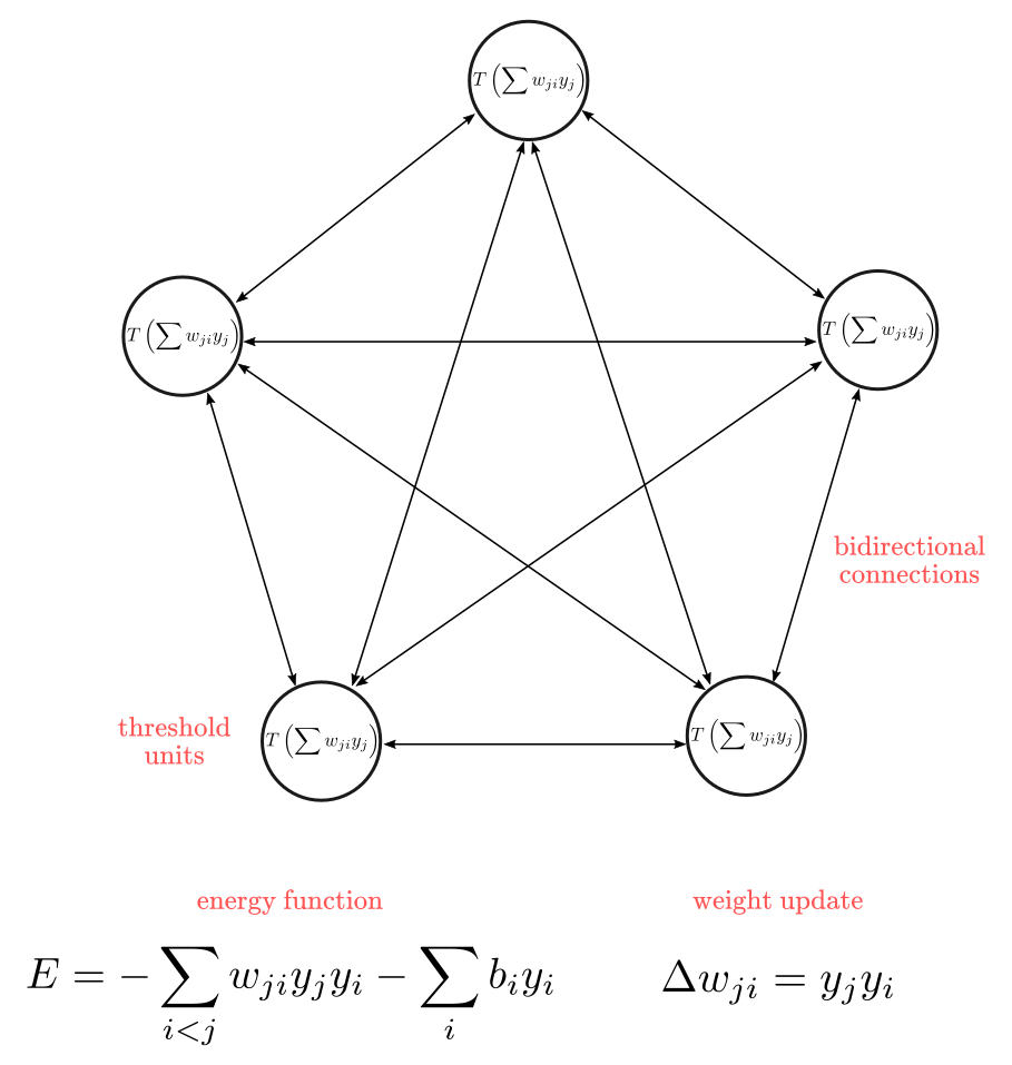
Hopfield network’s idea is that each configuration of binary-values $C$ in the network is associated with a global energy value $-E$. Here is a simplified picture of the training process: imagine you have a network with five neurons with a configuration of $C_1=(0, 1, 0, 1, 0)$. Now, imagine $C_1$ yields a global energy-value $E_1= 2$ (following the energy function formula). Your goal is to minimize $E$ by changing one element of the network $c_i$ at a time. By using the weight updating rule $\Delta w$, you can subsequently get a new configuration like $C_2=(1, 1, 0, 1, 0)$, as new weights will cause a change in the activation values $(0,1)$. If $C_2$ yields a lower value of $E$, let’s say, $1.5$, you are moving in the right direction. If you keep iterating with new configurations the network will eventually “settle” into a global energy minimum (conditioned to the initial state of the network).

A fascinating aspect of Hopfield networks, besides the introduction of recurrence, is that is closely based in neuroscience research about learning and memory, particularly Hebbian learning (Hebb, 1949). In fact, Hopfield (1982) proposed this model as a way to capture memory formation and retrieval. The idea is that the energy-minima of the network could represent the formation of a memory, which further gives rise to a property known as content-addressable memory (CAM). Here is the idea with a computer analogy: when you access information stored in the random access memory of your computer (RAM), you give the “address” where the “memory” is located to retrieve it. CAM works the other way around: you give information about the content you are searching for, and the computer should retrieve the “memory”. This is great because this works even when you have partial or corrupted information about the content, which is a much more realistic depiction of how human memory works. It is similar to doing a google search. Just think in how many times you have searched for lyrics with partial information, like “song with the beeeee bop ba bodda bope!”.

It is important to highlight that the sequential adjustment of Hopfield networks is not driven by error correction: there isn’t a “target” as in supervised-based neural networks. Hopfield networks are systems that “evolve” until they find a stable low-energy state. If you “perturb” such a system, the system will “re-evolve” towards its previous stable-state, similar to how those inflatable “Bop Bags” toys get back to their initial position no matter how hard you punch them. It is almost like the system “remembers” its previous stable-state (isn’t?). This ability to “return” to a previous stable-state after the perturbation is why they serve as models of memory.

Elman Network

Although Hopfield networks where innovative and fascinating models, the first successful example of a recurrent network trained with backpropagation was introduced by Jeffrey Elman, the so-called Elman Network (Elman, 1990). Elman was a cognitive scientist at UC San Diego at the time, part of the group of researchers that published the famous PDP book.

In 1990, Elman published “Finding Structure in Time”, a highly influential work for in cognitive science. Elman was concerned with the problem of representing “time” or “sequences” in neural networks. In his view, you could take either an “explicit” approach or an “implicit” approach. The explicit approach represents time spacially. Consider a vector $x = [x_1,x_2 \cdots, x_n]$, where element $x_1$ represents the first value of a sequence, $x_2$ the second element, and $x_n$ the last element. Hence, the spacial location in $\bf{x}$ is indicating the temporal location of each element. You can think about elements of $\bf{x}$ as sequences of words or actions, one after the other, for instance: $x^1=[Sound, of, the, funky, drummer]$ is a sequence of length five. Elman saw several drawbacks to this approach. First, although $\bf{x}$ is a sequence, the network still needs to represent the sequence all at once as an input, this is, a network would need five input neurons to process $x^1$. Second, it imposes a rigid limit on the duration of pattern, in other words, the network needs a fixed number of elements for every input vector $\bf{x}$: a network with five input units, can’t accommodate a sequence of length six. True, you could start with a six input network, but then shorter sequences would be misrepresented since mismatched units would receive zero input. This is a problem for most domains where sequences have a variable duration. Finally, it can’t easily distinguish relative temporal position from absolute temporal position. Consider the sequence $s = [1, 1]$ and a vector input length of four bits. Such a sequence can be presented in at least three variations:

$x_1 = [0, 1, 1, 0]\\ x_2 = [0, 0, 1, 1]\\ x_3 = [1, 1, 0, 0]$

Here, $\bf{x_1}$, $\bf{x_2}$, and $\bf{x_3}$ are instances of $\bf{s}$ but spacially displaced in the input vector. Geometrically, those three vectors are very different from each other (you can compute similarity measures to put a number on that), although representing the same instance. Even though you can train a neural net to learn those three patterns are associated with the same target, their inherent dissimilarity probably will hinder the network’s ability to generalize the learned association.

The implicit approach represents time by its effect in intermediate computations. To do this, Elman added a context unit to save past computations and incorporate those in future computations. In short, memory. Elman based his approach in the work of Michael I. Jordan on serial processing (1986). Jordan’s network implements recurrent connections from the network output $\hat{y}$ to its hidden units $h$, via a “memory unit” $\mu$ (equivalent to Elman’s “context unit”) as depicted in Figure 2. In short, the memory unit keeps a running average of all past outputs: this is how the past history is implicitly accounted for on each new computation. There is no learning in the memory unit, which means the weights are fixed to $1$.

Figure 2: Jordan Network

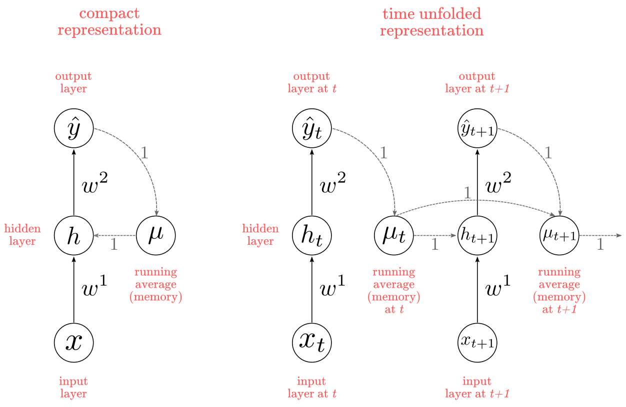
Note: Jordan’s network diagrams exemplifies the two ways in which recurrent nets are usually represented. On the left, the compact format depicts the network structure as a circuit. On the right, the unfolded representation incorporates the notion of time-steps calculations. The unfolded representation also illustrates how a recurrent network can be constructed in a pure feed-forward fashion, with as many layers as time-steps in your sequence. One key consideration is that the weights will be identical on each time-step (or layer). Keep this unfolded representation in mind as will become important later.

Elman’s innovation was twofold: recurrent connections between hidden units and memory (context) units, and trainable parameters from the memory units to the hidden units. Memory units now have to “remember” the past state of hidden units, which means that instead of keeping a running average, they “clone” the value at the previous time-step $t-1$. Memory units also have to learn useful representations (weights) for encoding temporal properties of the sequential input. Figure 3 summarizes Elman’s network in compact and unfolded fashion.

Figure 3: Elman Network

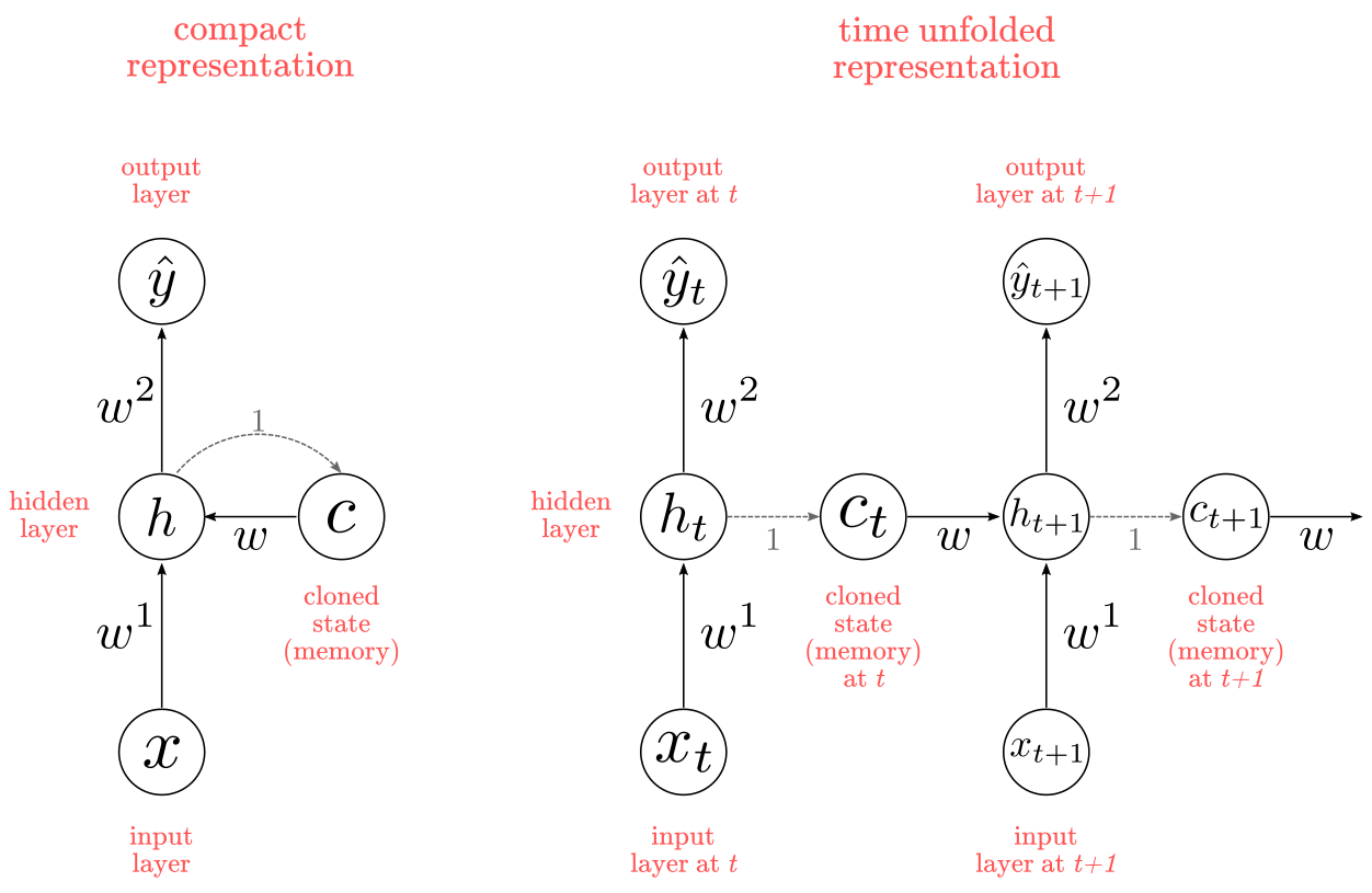
Note: there is something curious about Elman’s architecture. What it is the point of “cloning” $h$ into $c$ at each time-step? You could bypass $c$ altogether by sending the value of $h_t$ straight into $h_{t+1}$, wich yield mathematically identical results. The most likely explanation for this was that Elman’s starting point was Jordan’s network, which had a separated memory unit. Regardless, keep in mind we don’t need $c$ units to design a functionally identical network.

Elman performed multiple experiments with this architecture demonstrating it was capable to solve multiple problems with a sequential structure: a temporal version of the XOR problem; learning the structure (i.e., vowels and consonants sequential order) in sequences of letters; discovering the notion of “word”, and even learning complex lexical classes like word order in short sentences. Let’s briefly explore the temporal XOR solution as an exemplar. Table 1 shows the XOR problem:

Table 1: Truth Table For XOR Function

$x_1$	$x_2$	$y$
0	0	0
0	1	1
1	0	1
1	1	0

Here is a way to transform the XOR problem into a sequence. Consider the following vector:

$s= [1, 0, 1, 0, 0, 0, 0, 1, 1, 1, 1, 0, 1, 0, 1,...]$

In $\bf{s}$, the first and second elements, $s_1$ and $s_2$, represent $x_1$ and $x_2$ inputs of Table 1, whereas the third element, $s_3$, represents the corresponding output $y$. This pattern repeats until the end of the sequence $s$ as shown in Figure 4.

Figure 4: Temporal XOR

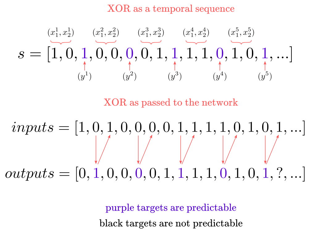
Elman trained his network with a 3,000 elements sequence for 600 iterations over the entire dataset, on the task of predicting the next item $s_{t+1}$ of the sequence $s$, meaning that he fed inputs to the network one by one. He showed that error pattern followed a predictable trend: the mean squared error was lower every 3 outputs, and higher in between, meaning the network learned to predict the third element in the sequence, as shown in Chart 1 (the numbers are made up, but the pattern is the same found by Elman (1990)).

import numpy as np
import pandas as pd
import altair as alt

s = pd.DataFrame({"MSE": [0.35, 0.15, 0.30, 0.27, 0.14, 0.40, 0.35, 0.12, 0.36, 0.31, 0.15, 0.32],
                  "cycle": np.arange(1, 13)})
alt.Chart(s).mark_line().encode(x="cycle", y="MSE").properties(title='Chart 1')

An immediate advantage of this approach is the network can take inputs of any length, without having to alter the network architecture at all.

In the same paper, Elman showed that the internal (hidden) representations learned by the network grouped into meaningful categories, this is, semantically similar words group together when analyzed with hierarchical clustering. This was remarkable as demonstrated the utility of RNNs as a model of cognition in sequence-based problems.

Interlude: vanishing and exploding gradients in RNNs

Turns out, training recurrent neural networks is hard. Considerably harder than multilayer-perceptrons. When faced with the task of training very deep networks, like RNNs, the gradients have the impolite tendency of either (1) vanishing, or (2) exploding (Bengio et al, 1994; Pascanu et al, 2012). Recall that RNNs can be unfolded so that recurrent connections follow pure feed-forward computations. This unrolled RNN will have as many layers as elements in the sequence. Thus, a sequence of 50 words will be unrolled as an RNN of 50 layers (taking “word” as a unit).

Concretely, the vanishing gradient problem will make close to impossible to learn long-term dependencies in sequences. Let’s say you have a collection of poems, where the last sentence refers to the first one. Such a dependency will be hard to learn for a deep RNN where gradients vanish as we move backward in the network. The exploding gradient problem will completely derail the learning process. In very deep networks this is often a problem because more layers amplify the effect of large gradients, compounding into very large updates to the network weights, to the point values completely blow up.

Here is the intuition for the mechanics of gradient vanishing: when gradients begin small, as you move backward through the network computing gradients, they will get even smaller as you get closer to the input layer. Consequently, when doing the weight update based on such gradients, the weights closer to the output layer will obtain larger updates than weights closer to the input layer. This means that the weights closer to the input layer will hardly change at all, whereas the weights closer to the output layer will change a lot. This is a serious problem when earlier layers matter for prediction: they will keep propagating more or less the same signal forward because no learning (i.e., weight updates) will happen, which may significantly hinder the network performance.

Here is the intuition for the mechanics of gradient explosion: when gradients begin large, as you move backward through the network computing gradients, they will get even larger as you get closer to the input layer. Consequently, when doing the weight update based on such gradients, the weights closer to the input layer will obtain larger updates than weights closer to the output layer. Learning can go wrong really fast. Recall that the signal propagated by each layer is the outcome of taking the product between the previous hidden-state and the current hidden-state. If the weights in earlier layers get really large, they will forward-propagate larger and larger signals on each iteration, and the predicted output values will spiral-up out of control, making the error $y-\hat{y}$ so large that the network will be unable to learn at all. In fact, your computer will “overflow” quickly as it would unable to represent numbers that big. Very dramatic.

The mathematics of gradient vanishing and explosion gets complicated quickly. If you want to delve into the mathematics see Bengio et all (1994), Pascanu et all (2012), and Philipp et all (2017).

For our purposes, I’ll give you a simplified numerical example for intuition. Consider the task of predicting a vector $y = \begin{bmatrix} 1 & 1 \end{bmatrix}$, from inputs $x = \begin{bmatrix} 1 & 1 \end{bmatrix}$, with a multilayer-perceptron with 5 hidden layers and tanh activation functions. We have two cases:

the weight matrix $W_l$ is initialized to large values $w_{ij} = 2$
the weight matrix $W_s$ is initialized to small values $w_{ij} = 0.02$

Now, let’s compute a single forward-propagation pass:

import numpy as np

x = np.array([[1],[1]])
W_l = np.array([[2, 2],
                [2, 2]])

h1 = np.tanh(W_l @ x)
h2 = np.tanh(W_l @ h1)
h3 = np.tanh(W_l @ h2)
h4 = np.tanh(W_l @ h3)
h5 = np.tanh(W_l @ h4)
y_hat = (W_l @ h5)
print(f'output for large initial weights: \n {y_hat}')

output for large initial weights: 
 [[3.99730269]
 [3.99730269]]

x = np.array([[1],[1]])
W_s = np.array([[0.02, 0.02],
                [0.02, 0.02]])

h1 = np.tanh(W_s @ x)
h2 = np.tanh(W_s @ h1)
h3 = np.tanh(W_s @ h2)
h4 = np.tanh(W_s @ h3)
h5 = np.tanh(W_s @ h4)
y_hat = (W_s @ h5)
print(f'output for small initial weights: \n {y_hat}')

output for small initial weights: 
 [[4.09381337e-09]
 [4.09381337e-09]]

We see that for $W_l$ the output $\hat{y}\approx4$, whereas for $W_s$ the output $\hat{y} \approx 0$. Why does this matter? We haven’t done the gradient computation but you can probably anticipate what it’s going to happen: for the $W_l$ case, the gradient update is going to be very large, and for the $W_s$ very small. If you keep cycling through forward and backward passes these problems will become worse, leading to gradient explosion and vanishing respectively.

Long Short-Term Memory Network

Several challenges difficulted progress in RNN in the early ’90s (Hochreiter & Schmidhuber, 1997; Pascanu et al, 2012). In addition to vanishing and exploding gradients, we have the fact that the forward computation is slow, as RNNs can’t compute in parallel: to preserve the time-dependencies through the layers, each layer has to be computed sequentially, which naturally takes more time. Elman networks proved to be effective at solving relatively simple problems, but as the sequences scaled in size and complexity, this type of network struggle.

Several approaches were proposed in the ’90s to address the aforementioned issues like time-delay neural networks (Lang et al, 1990), simulated annealing (Bengio et al., 1994), and others. The architecture that really moved the field forward was the so-called Long Short-Term Memory (LSTM) Network, introduced by Sepp Hochreiter and Jurgen Schmidhuber in 1997. As the name suggests, the defining characteristic of LSTMs is the addition of units combining both short-memory and long-memory capabilities.

In LSTMs, instead of having a simple memory unit “cloning” values from the hidden unit as in Elman networks, we have a (1) cell unit (a.k.a., memory unit) which effectively acts as long-term memory storage, and (2) a hidden-state which acts as a memory controller. These two elements are integrated as a circuit of logic gates controlling the flow of information at each time-step. Understanding the notation is crucial here, which is depicted in Figure 5.

Figure 5: LSTM architecture

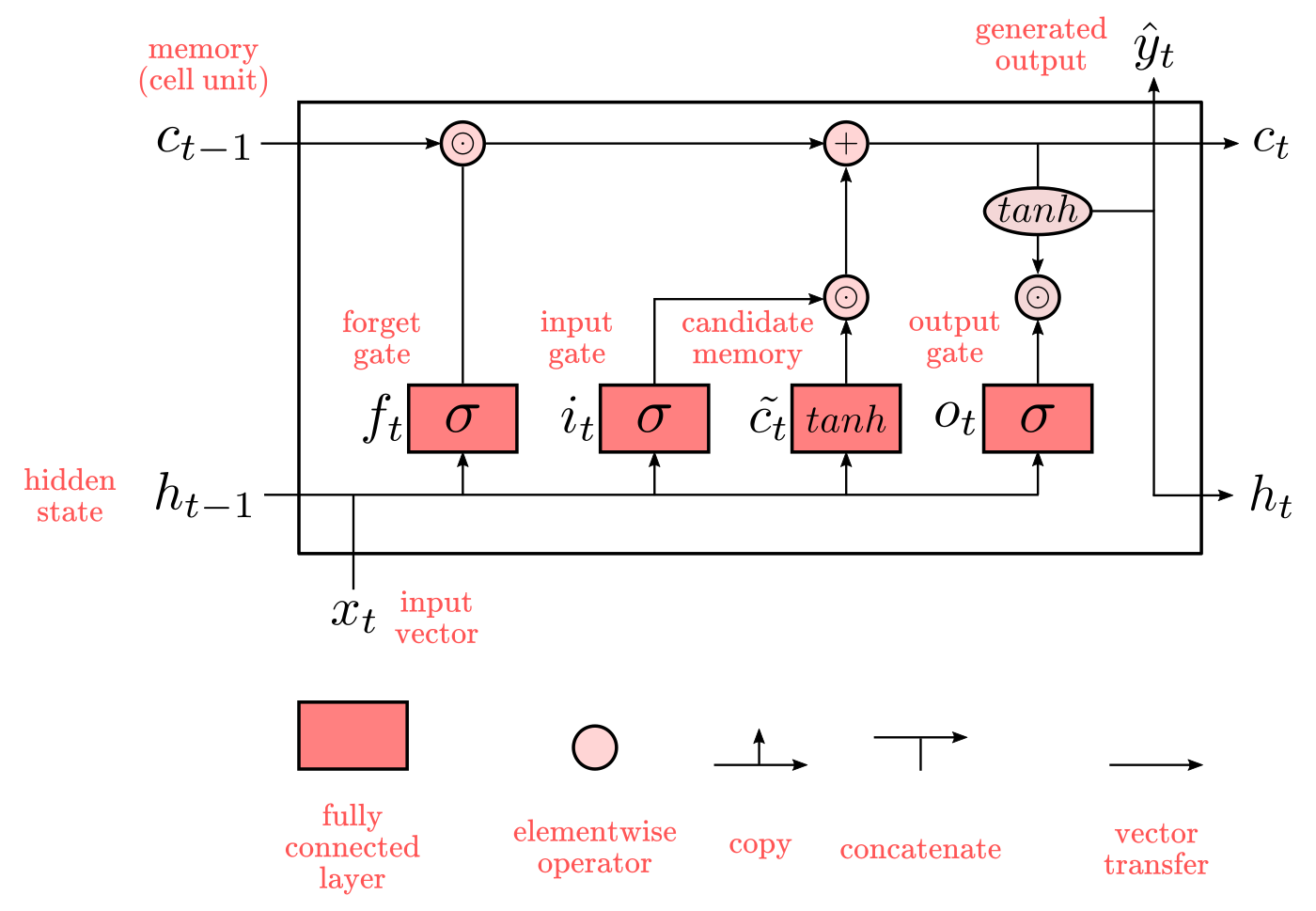
In LSTMs $x_t$, $h_t$, and $c_t$ represent vectors of values. Lightish-pink circles represent element-wise operations, and darkish-pink boxes are fully-connected layers with trainable weights. The top part of the diagram acts as a memory storage, whereas the bottom part has a double role: (1) passing the hidden-state information from the previous time-step $t-1$ to the next time step $t$, and (2) to regulate the influx of information from $x_t$ and $h_{t-1}$ into the memory storage, and the outflux of information from the memory storage into the next hidden state $h-t$. The second role is the core idea behind LSTM. You can think about it as making three decisions at each time-step:

Is the old information $c_{t-1}$ worth to keep in my memory storage $c_t$? If so, let the information pass, otherwise, “forget” such information. This is controlled by the forget gate.
Is this new information (inputs) worth to be saved into my memory storage $c_t$? If so, let information flow into $c_t$. This is controlled by the input gate and the candidate memory cell.
What elements of the information saved in my memory storage $c_t$ are relevant for the computation of the next hidden-state $h_t$? Select them from $c_t$, combine them new hidden-state output, and let them pass into the next hidden-state $h_t$. This is controlled by the output gate and the tanh function.

Decisions 1 and 2 will determine the information that keeps flowing through the memory storage at the top. Decision 3 will determine the information that flows to the next hidden-state at the bottom. The conjunction of these decisions sometimes is called “memory block”. Now, keep in mind that this sequence of decision is just a convenient interpretation of LSTM mechanics. In practice, the weights are the ones determining what each function ends up doing, which may or may not fit well with human intuitions or design objectives.

Figure 6: LSTM as a sequence of decisions

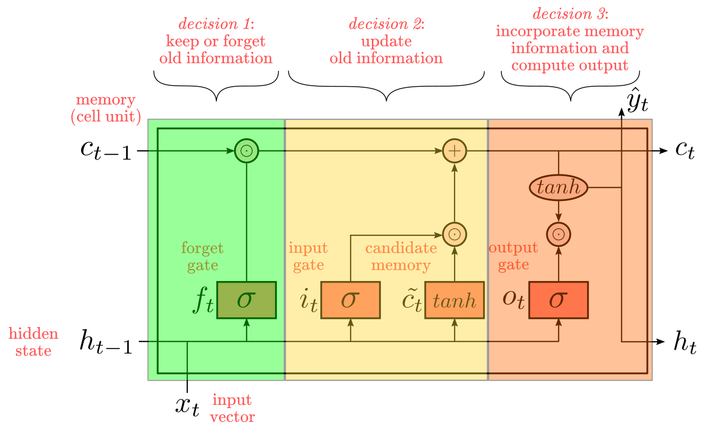
To put LSTMs in context, imagine the following simplified scenerio: we are trying to predict the next word in a sequence. Let’s say, squences are about sports. From past sequences, we saved in the memory block the type of sport: “soccer”. For the current sequence, we receive a phrase like “A basketball player…”. In such a case, we first want to “forget” the previous type of sport “soccer” (decision 1) by multplying $c_{t-1} \odot f_t$. Next, we want to “update” memory with the new type of sport, “basketball” (decision 2), by adding $c_t = (c_{t-1} \odot f_t) + (i_t \odot \tilde{c_t})$. Finally, we want to output (decision 3) a verb relevant for “A basketball player…”, like “shoot” or “dunk” by $\hat{y_t} = softmax(W_{hz}h_t + b_z)$.

LSTMs long-term memory capabilities make them good at capturing long-term dependencies. The memory cell effectively counteracts the vanishing gradient problem at preserving information as long the forget gate does not “erase” past information (Graves, 2012). All the above make LSTMs sere](https://en.wikipedia.org/wiki/Long_short-term_memory#Applications)). For instance, when you use Google’s Voice Transcription services an RNN is doing the hard work of recognizing your voice.uccessful in practical applications in sequence-modeling (see a list here). For instance, when you use Google’s Voice Transcription services an RNN is doing the hard work of recognizing your voice.

RNNs and cognition

As with Convolutional Neural Networks, researchers utilizing RNN for approaching sequential problems like natural language processing (NLP) or time-series prediction, do not necessarily care about (although some might) how good of a model of cognition and brain-activity are RNNs. What they really care is about solving problems like translation, speech recognition, and stock market prediction, and many advances in the field come from pursuing such goals. Still, RNN has many desirable traits as a model of neuro-cognitive activity, and have been prolifically used to model several aspects of human cognition and behavior: child behavior in an object permanence tasks (Munakata et al, 1997); knowledge-intensive text-comprehension (St. John, 1992); processing in quasi-regular domains, like English word reading (Plaut et al., 1996); human performance in processing recursive language structures (Christiansen & Chater, 1999); human sequential action (Botvinick & Plaut, 2004); movement patterns in typical and atypical developing children (Muñoz-Organero et al., 2019). And many others. Neuroscientists have used RNNs to model a wide variety of aspects as well (for reviews see Barak, 2017, Güçlü & van Gerven, 2017, Jarne & Laje, 2019). Overall, RNN has demonstrated to be a productive tool for modeling cognitive and brain function, in distributed representations paradigm.

Mathematical formalization

There are two mathematically complex issues with RNNs: (1) computing hidden-states, and (2) backpropagation. The rest are common operations found in multilayer-perceptrons. LSTMs and its many variants are the facto standards when modeling any kind of sequential problem. Elman networks can be seen as a simplified version of an LSTM, so I’ll focus my attention on LSTMs for the most part. My exposition is based on a combination of sources that you may want to review for extended explanations (Bengio et al., 1994; Hochreiter & Schmidhuber, 1997; Graves, 2012; Chen, 2016; Zhang et al., 2020).

The LSTM architecture can be desribed by:

Forward pass:

non-linear forget function
non-linear input function
non-linear candidate-memory function
non-linear output function
memory cell function
non-linear hidden-state function
softmax function (output)

Backward pass:

Cost-function
Learning procedure (backpropagation)

Following the indices for each function requires some definitions. I’ll assume we have $h$ hidden units, training sequences of size $n$, and $d$ input units.

$\text{input-units} = x_i \in \mathbb{R}^d \\ \text{training-sequence} = s_i \in \mathbb{R}^n \\ \text{output-class} = y_i \in \mathbb{R}^k \\ \text{Input-layer} = X_t \in \mathbb{R}^{n\times d} \\ \text{hidden-layer} = H_t \in \mathbb{R}^{n\times h}$

Forget function

The forget function is a sigmoidal mapping combining three elements: input vector $x_t$, past hidden-state $h_{t-1}$, and a bias term $b_f$. We didn’t mentioned the bias before, but it is the same bias that all neural networks incorporate, one for each unit in $f$. More formally:

$f_t = \sigma(W_{xf}x_t + W_{hf}h_{t-1} + b_f)$

Each matrix $W$ has dimensionality equal to (number of incoming units, number for connected units). For example, $W_{xf}$ refers to $W_{input-units, forget-units}$. Keep this in mind to read the indices of the $W$ matrices for subsequent definitions.

Here is an important insight: What would it happen if $f_t = 0$? If you look at the diagram in Figure 6, $f_t$ performs an elementwise multiplication of each element in $c_{t-1}$, meaning that every value would be reduced to $0$. In short, the network would completely “forget” past states. Naturally, if $f_t = 1$, the network would keep its memory intact.

Input function and Candidate memory function

The input function is a sigmoidal mapping combining three elements: input vector $x_t$, past hidden-state $h_{t-1}$, and a bias term $b_f$. It’s defined as:

$i_t = \sigma(W_{xi}x_t + W_{hi}h_{t-1} + b_i)$

The candidate memory function is an hyperbolic tanget function combining the same elements that $i_t$. It’s defined as:

$\tilde{c}_t = tanh(W_{xc}x_t + W_{hc}h_{t-1} + b_c)$

Both functions are combined to update the memory cell.

Output function

The output function is a sigmoidal mapping combining three elements: input vector $x_t$, past hidden-state $h_{t-1}$, and a bias term $b_f$. Is defined as:

$o_t = \sigma(W_{xo}x_t + W_{ho}h_{t-1} + b_o)$

Memory cell function

The memory cell function (what I’ve been calling “memory storage” for conceptual clarity), combines the effect of the forget function, input function, and candidate memory function. It’s defined as:

$c_t = (c_{t-1} \odot f_t) + (i_t \odot \tilde{c_t})$

Where $\odot$ implies an elementwise multiplication (instead of the usual dot product). This expands to:

$c_t = (c_{t-1} \odot \sigma(W_{xf}x_t + W_{hf}h_{t-1} + b_f)) + (\sigma(W_{xi}x_t + W_{hi}h_{t-1} + b_i) \odot tanh(W_{xc}x_t + W_{hc}h_{t-1} + b_c))$

Hidden-state function

The next hidden-state function combines the effect of the output function and the contents of the memory cell scaled by a tanh function. It is defined as:

$h_t = O_t \odot tanh(c_t)$

Output function

The output function will depend upon the problem to be approached. For our our purposes, we will assume a multi-class problem, for which the softmax function is appropiated. For this, we first pass the hidden-state by a linear function, and then the softmax as:

$z_t = (W_{hz}h_t + b_z)\\ \hat{y}_t = softmax(z_t) = \frac{e^{z_t}}{\sum_{j=1}^K e^{z_j}}$

The softmax computes the exponent for each $z_t$ and then normalized by dividing by the sum of every output value exponentiated. In this manner, the output of the softmax can be interpreted as the likelihood value $p$.

Cost function

As with the output function, the cost function will depend upon the problem. For regression problems, the Mean-Squared Error can be used. For our purposes (classification), the cross-entropy function is appropriated. It’s defined as:

$E_i = - \sum_t y_ilog(p_i)$

Where $y_i$ is the true label for the $ith$ output unit, and $log(p_i)$ is the log of the softmax value for the $ith$ output unit. The summation indicates we need to aggregate the cost at each time-step.

Learning procedure: Backpropagation Through Time (BPTT)

Originally, Hochreiter and Schmidhuber (1997) trained LSTMs with a combination of approximate gradient descent computed with a combination of real-time recurrent learning and backpropagation through time (BPTT). Nevertheless, LSTM can be trained with pure backpropagation. Following Graves (2012), I’ll only describe BTT because is more accurate, easier to debug and to describe.

Note: we call it backpropagation through time because of the sequential time-dependent structure of RNNs. Recall that each layer represents a time-step, and forward propagation happens in sequence, one layer computed after the other. Hence, when we backpropagate, we do the same but backward (i.e., “through time”).

Figure 7: Three-layer simplified RNN

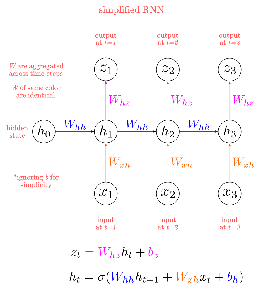
I reviewed backpropagation for a simple multilayer perceptron here. Nevertheless, I’ll sketch BPTT for the simplest case as shown in Figure 7, this is, with a generic non-linear hidden-layer similar to Elman network without “context units” (some like to call it “vanilla” RNN, which I avoid because I believe is derogatory against vanilla!). This exercise will allow us to review backpropagation and to understand how it differs from BPTT. We begin by defining a simplified RNN as:

$z_t = W_{hz}h_t + b_z\\ h_t = \sigma(W_{hh}h_{t-1} + W_{xh}x_t+b_h)$

Where $h_t$ and $z_t$ indicates a hidden-state (or layer) and the output respectively. Therefore, we have to compute gradients w.r.t. five sets of weights: ${W_{hz}, W_{hh}, W_{xh}, b_z, b_h}$.

First, consider the error derivatives w.r.t. $W_{hz}$ at time $t$, the weight matrix for the linear function at the output layer. Recall that $W_{hz}$ is shared across all time-steps, hence, we can compute the gradients at each time step and then take the sum as:

$\frac{\partial{E}}{\partial{W_{hz}}} = \sum_t\frac{\partial{E}}{\partial{z_t}} \frac{\partial{z_t}}{\partial{W_{hz}}}$

Same for the bias term:

$\frac{\partial{E}}{\partial{b_z}} = \sum_t\frac{\partial{E}}{\partial{z_t}} \frac{\partial{z_t}}{\partial{b_z}}$

That part is straightforward. The issue arises when we try to compute the gradients w.r.t. the wights $W_{hh}$ in the hidden layer. Consider a three layer RNN (i.e., unfolded over three time-steps). In such a case, we have:

$E_3$ depens on $z_3$
$z_3$ depends on $h_3$
$h_3$ depens on $h_2$
$h_2$ depens on $h_1$
$h_1$ depens on $h_0$, where $h_0$ is a random starting state.

Now, we have that $E_3$ w.r.t to $h_3$ becomes:

$\frac{\partial{E_3}}{\partial{W_{hh}}} = \frac{\partial{E_3}}{\partial{z_3}} \frac{\partial{z_3}}{\partial{h_3}} \frac{\partial{h_3}}{\partial{W_{hh}}}$

The issue here is that $h_3$ depends on $h_2$, since according to our definition, the $W_{hh}$ is multiplied by $h_{t-1}$, meaning we can’t compute $\frac{\partial{h_3}}{\partial{W_{hh}}}$ directly. Othewise, we would be treating $h_2$ as a constant, which is incorrect: is a function. What we need to do is to compute the gradients separately: the direct contribution of ${W_{hh}}$ on $E$ and the indirect contribution via $h_2$. Following the rules of calculus in multiple variables, we compute them independently and add them up together as:

Again, we have that we can’t compute $\frac{\partial{h_2}}{\partial{W_{hh}}}$ directly. Following the same procedure, we have that our full expression becomes:

$\frac{\partial{E_3}}{\partial{W_{hh}}} = \frac{\partial{E_3}}{\partial{z_3}} \frac{\partial{z_3}}{\partial{h_3}} \frac{\partial{h_3}}{\partial{W_{hh}}}+ \frac{\partial{E_3}}{\partial{z_3}} \frac{\partial{z_3}}{\partial{h_3}} \frac{\partial{h_3}}{\partial{h_2}} \frac{\partial{h_2}}{\partial{W_{hh}}}+ \frac{\partial{E_3}}{\partial{z_3}} \frac{\partial{z_3}}{\partial{h_3}} \frac{\partial{h_3}}{\partial{h_2}} \frac{\partial{h_2}}{\partial{h_1}} \frac{\partial{h_1}}{\partial{W_{hh}}}$

Essentially, this means that we compute and add the contribution of $W_{hh}$ to $E$ at each time-step. The expression for $b_h$ is the same:

$\frac{\partial{E_3}}{\partial{b_h}} = \frac{\partial{E_3}}{\partial{z_3}} \frac{\partial{z_3}}{\partial{h_3}} \frac{\partial{h_3}}{\partial{b_h}}+ \frac{\partial{E_3}}{\partial{z_3}} \frac{\partial{z_3}}{\partial{h_3}} \frac{\partial{h_3}}{\partial{h_2}} \frac{\partial{h_2}}{\partial{b_h}}+ \frac{\partial{E_3}}{\partial{z_3}} \frac{\partial{z_3}}{\partial{h_3}} \frac{\partial{h_3}}{\partial{h_2}} \frac{\partial{h_2}}{\partial{h_1}} \frac{\partial{h_1}}{\partial{b_h}}$

Finally, we need to compute the gradients w.r.t. $W_{xh}$. Here, again, we have to add the contributions of $W_{xh}$ via $h_3$, $h_2$, and $h_1$:

$\frac{\partial{E_3}}{\partial{W_{xh}}} = \frac{\partial{E_3}}{\partial{z_3}} \frac{\partial{z_3}}{\partial{h_3}} \frac{\partial{h_3}}{\partial{W_{xh}}}+ \frac{\partial{E_3}}{\partial{z_3}} \frac{\partial{z_3}}{\partial{h_3}} \frac{\partial{h_3}}{\partial{h_2}} \frac{\partial{h_2}}{\partial{W_{xh}}}+ \frac{\partial{E_3}}{\partial{z_3}} \frac{\partial{z_3}}{\partial{h_3}} \frac{\partial{h_3}}{\partial{h_2}} \frac{\partial{h_2}}{\partial{h_1}} \frac{\partial{h_1}}{\partial{W_{xh}}}$

That’s for BPTT for a simple RNN. The math reviewed here generalizes with minimal changes to more complex architectures as LSTMs. Actually, the only difference regarding LSTMs, is that we have more weights to differentiate for. Instead of a single generic $W_{hh}$, we have $W$ for all the gates: forget, input, output, and candidate cell. The rest remains the same. For a detailed derivation of BPTT for the LSTM see Graves (2012) and Chen (2016).

Interlude: Sequence-data representation

Working with sequence-data, like text or time-series, requires to pre-process it in a manner that is “digestible” for RNNs. As with any neural network, RNN can’t take raw text as an input, we need to parse text sequences and then “map” them into vectors of numbers. Here I’ll briefly review these issues to provide enough context for our example applications. For an extended revision please refer to Jurafsky and Martin (2019), Goldberg (2015), Chollet (2017), and Zhang et al (2020).

Parsing can be done in multiple manners, the most common being:

Using word as a unit, which each word represented as a vector
Using character as a unit, with each character represented as a vector
Using n-grams of words or characters as a unit, with each n-gram represented as a vector. N-grams are sets of words or characters of size “N” or less.

The process of parsing text into smaller units is called “tokenization”, and each resulting unit is called a “token”, the top pane in Figure 8 displays a sketch of the tokenization process.

Figure 8: Tokenization

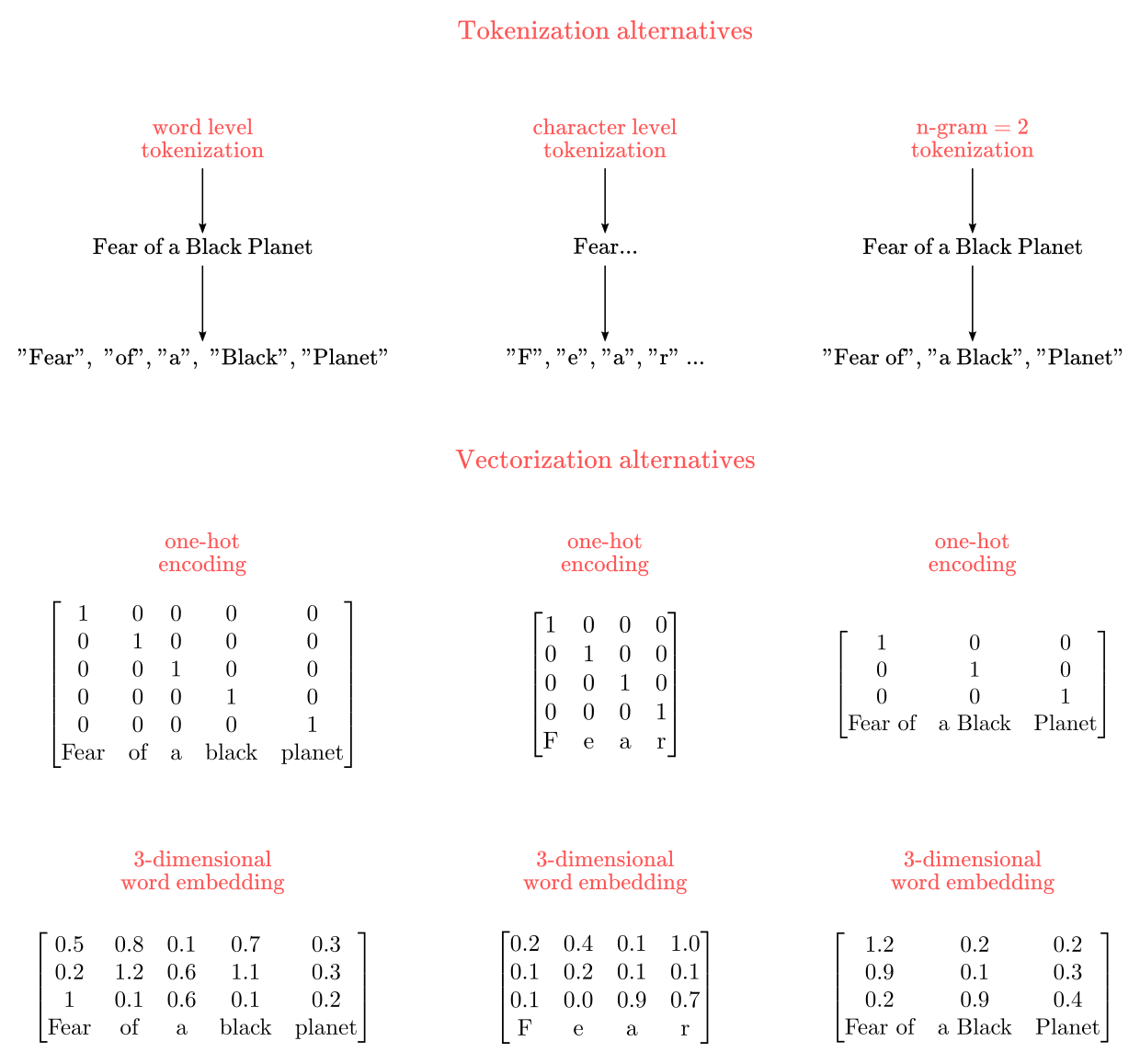
Once a corpus of text has been parsed into tokens, we have to map such tokens into numerical vectors. Two common ways to do this are one-hot encoding approach and the word embeddings approach, as depicted in the bottom pane of Figure 8. We used one-hot encodings to transform the MNIST class-labels into vectors of numbers for classification in the CovNets blogpost. In a one-hot encoding vector, each token is mapped into a unique vector of zeros and ones. The vector size is determined by the vocabullary size. For instance, for the set $x= {“cat”, “dog”, “ferret”}$, we could use a 3-dimensional one-hot encoding as:

$\text{cat}= \begin{bmatrix} 1 \\ 0 \\ 0 \end{bmatrix}, \text{dog}= \begin{bmatrix} 0 \\ 1 \\ 0 \end{bmatrix}, \text{ferret}= \begin{bmatrix} 0 \\ 0 \\ 1 \end{bmatrix}$

One-hot encodings have the advantages of being straightforward to implement and to provide a unique identifier for each token. Its main disadvantage is that tends to create really sparse and high-dimensional representations for a large corpus of texts. For instance, if you tried a one-hot encoding for 50,000 tokens, you’d end up with a 50,000x50,000-dimensional matrix, which may be unpractical for most tasks.

Word embeddings represent text by mapping tokens into vectors of real-valued numbers instead of only zeros and ones. This significantly increments the representational capacity of vectors, reducing the required dimensionality for a given corpus of text compared to one-hot encodings. For instance, 50,000 tokens could be represented by as little as 2 or 3 vectors (although the representation may not be very good). Taking the same set $x$ as before, we could have a 2-dimensional word embedding like:

$\text{cat}= \begin{bmatrix} 0.1 \\ 0.8 \end{bmatrix}, \text{dog}= \begin{bmatrix} 0.2 \\ 1 \end{bmatrix}, \text{ferret}= \begin{bmatrix} 0.6 \\ 0.2 \end{bmatrix}$

You may be wondering why to bother with one-hot encodings when word embeddings are much more space-efficient. The main issue with word-embedding is that there isn’t an obvious way to map tokens into vectors as with one-hot encodings. For instance, you could assign tokens to vectors at random (assuming every token is assigned to a unique vector). The problem with such approach is that the semantic structure in the corpus is broken. Ideally, you want words of similar meaning mapped into similar vectors. We can preserve the semantic structure of a text corpus in the same manner as everything else in machine learning: by learning from data. There are two ways to do this:

Learning the word embeddings at the same time you train the RNN.
Utilizing pretrained word embeddings, this is, embeddings learned in a different task. This is a form of “transfer learning”.

Learning word embeddings for your task is advisable as semantic relationships among words tend to be context dependent. For instance, “exploitation” in the context of mining is related to resource “extraction”, hence relative neutral. But, “exploitation” in the context of labor rights is related to the idea of “abuse”, hence a negative connotation. This is more critical when we are dealing with different languages. Nevertheless, learning embeddings for every task sometimes is impractical, either because your corpus is too “small” (i.e., not enough data to extract semantic relationships), or too “large” (i.e., you don’t have enough time and/or resources to learn the embeddings). Examples of freely accessible pretrained word embeddings are Google’s Word2vec and the Global Vectors for Word Representation (GloVe).

Code implementation

As in previous blogpost, I’ll use Keras to implement both (a modified version of) the Elman Network for the XOR problem and an LSTM for review prediction based on text-sequences.

Elman Network

By now, it may be clear to you that Elman networks are a simple RNN with two neurons, one for each input pattern, in the hidden-state. Originally, Elman trained his architecture with a truncated version of BPTT, meaning that only considered two time-steps for computing the gradients, $t$ and $t-1$. We will implement a modified version of Elman’s architecture bypassing the “context” unit (which does not alter the result at all) and utilizing BPTT instead of its truncated version.

Generating data

Nowadays, we don’t need to generate the 3,000 bits sequence that Elman used in his original work. We can simply generate a single pair of training and testing sets for the XOR problem as in Table 1, and pass the training sequence (length two) as the inputs, and the expected outputs as the target. This is very much alike any classification task. An important caveat is that simpleRNN layers in Keras expect an input tensor of shape (number-samples, timesteps, number-input-features). In our case, this has to be: number-samples= 4, timesteps=1, number-input-features=2. No separate encoding is necessary here because we are manually setting the input and output values to binary vector representations. Finally, we won’t worry about training and testing sets for this example, which is way to simple for that (we will do that for the next example).

# Libraries for this section

from keras.layers import Dense, SimpleRNN
from keras.models import Sequential
import altair as alt
import pandas as pd
import numpy as np

# features
X = np.array([[[0, 0, 1, 1]],
              [[0, 1, 0, 1]]]).T

# expected values
y = np.array([[0, 1, 1, 0]]).T

print(f'training data shape: {X.shape}')
print(f'targets data shape: {y.shape}')

training data shape: (4, 1, 2)
targets data shape: (4, 1)

Elman network architecture in Keras

Defining a (modified) in Keras is extremely simple as shown below.

# Define a network as a linear stack of layers
model = Sequential()

# Add a recurrent layer with 2 units
model.add(SimpleRNN(2, input_shape=(1, 2)))

# Add the output layer with a sigmoid activation
model.add(Dense(1, activation='tanh'))

The model summary shows that our architecture yields 13 trainable parameters.

model.summary()

Model: "sequential_1"
_________________________________________________________________
Layer (type)                 Output Shape              Param #   
=================================================================
simple_rnn_1 (SimpleRNN)     (None, 2)                 10        
_________________________________________________________________
dense_1 (Dense)              (None, 1)                 3         
=================================================================
Total params: 13
Trainable params: 13
Non-trainable params: 0
_________________________________________________________________

Elman network Application: XOR classification

Next, we compile and fit our model. I’ll utilize Adadelta (to avoid manually adjusting the learning rate) as the optimizer, and the Mean-Squared Error (as in Elman original work). I’ll train the model for 15,000 epochs over the 4 samples dataset.

model.compile(optimizer='Adadelta', 
              loss='mean_squared_error', 
              metrics=['acc'])
history = model.fit(X, y,
                    epochs=5000,
                    verbose=0)

Chart 2 shows the error curve (red, right axis), and the accuracy curve (blue, left axis) for each epoch.

alt.data_transformers.disable_max_rows()

loss = history.history['loss']
accuracy = history.history['acc']

df = pd.DataFrame({"accuracy":accuracy, "loss":loss, "time-step": np.arange(0, len(accuracy))})

base = alt.Chart(df).mark_line(color="blue").encode(x="time-step", y="accuracy")
loss = alt.Chart(df).mark_line(color="red").encode(x="time-step", y="loss")
(base  + loss).properties(title='Chart 2').resolve_scale(y='independent')

We see that accuracy goes to 100% in around 1,000 epochs (note that different runs may slightly change the results).

LSTM

In a strict sense, LSTM is a type of layer instead of a type of network. What I’ve calling LSTM networks is basically any RNN composed of LSTM layers. Most RNNs you’ll find in the wild (i.e., the internet) use either LSTMs or Gated Recurrent Units (GRU). We don’t cover GRU here since they are very similar to LSTMs and this blogpost is dense enough as it is. If you want to learn more about GRU see Cho et al (2014) and Chapter 9.1 from Zhang (2020).

For this section, I’ll base the code in the example provided by Chollet (2017) in chapter 6. As a side note, if you are interested in learning Keras in-depth, Chollet’s book is probably the best source since he is the creator of Keras library.

Reading and preprocessing data from Keras

If you are like me, you like to check the IMDB reviews before watching a movie. For this example, we will make use of the IMDB dataset, and Lucky us, Keras comes pre-packaged with it. The IMDB dataset comprises 50,000 movie reviews, 50% positive and 50% negative. Keras give access to a numerically encoded version of the dataset where each word is mapped to sequences of integers. We can download the dataset by running the following:

# Libraries for this section

import tensorflow as tf
from tensorflow.keras.layers import Dense, LSTM, Embedding
from tensorflow.keras.models import Sequential

from keras.datasets import imdb
from keras.preprocessing.sequence import pad_sequences
import altair as alt
import pandas as pd
import numpy as np

Note: This time I also imported Tensorflow, and from there Keras layers and models. Keras happens to be integrated with Tensorflow, as a high-level interface, so nothing important changes when doing this. Yet, there are some implementation issues with the optimizer that require importing from Tensorflow to work.

maxlen = 5000
(train_data, train_labels), (test_data, test_labels) = imdb.load_data(
num_words=maxlen)

The parameter num_words=5000 restrict the dataset to the top 5,000 most frequent words. We do this to avoid highly infrequent words. Often, infrequent words are either typos or words for which we don’t have enough statistical information to learn useful representations.

Data is downloaded as a (25000,) tuples of integers.

print(f'train-data shape: {train_data.shape}, train-labels shape: {train_labels.shape}')
print(f'test-data shape: {test_data.shape}, test-labels shape: {test_labels.shape} \n')
print(train_data[0],train_labels[0])

train-data shape: (25000,), train-labels shape: (25000,)
test-data shape: (25000,), test-labels shape: (25000,) 

[1, 14, 22, 16, 43, 530, 973, 1622, 1385, 65, 458, 4468, 66, 3941, 4, 173, 36, 256, 5, 25, 100, 43, 838, 112, 50, 670, 2, 9, 35, 480, 284, 5, 150, 4, 172, 112, 167, 2, 336, 385, 39, 4, 172, 4536, 1111, 17, 546, 38, 13, 447, 4, 192, 50, 16, 6, 147, 2025, 19, 14, 22, 4, 1920, 4613, 469, 4, 22, 71, 87, 12, 16, 43, 530, 38, 76, 15, 13, 1247, 4, 22, 17, 515, 17, 12, 16, 626, 18, 2, 5, 62, 386, 12, 8, 316, 8, 106, 5, 4, 2223, 2, 16, 480, 66, 3785, 33, 4, 130, 12, 16, 38, 619, 5, 25, 124, 51, 36, 135, 48, 25, 1415, 33, 6, 22, 12, 215, 28, 77, 52, 5, 14, 407, 16, 82, 2, 8, 4, 107, 117, 2, 15, 256, 4, 2, 7, 3766, 5, 723, 36, 71, 43, 530, 476, 26, 400, 317, 46, 7, 4, 2, 1029, 13, 104, 88, 4, 381, 15, 297, 98, 32, 2071, 56, 26, 141, 6, 194, 2, 18, 4, 226, 22, 21, 134, 476, 26, 480, 5, 144, 30, 2, 18, 51, 36, 28, 224, 92, 25, 104, 4, 226, 65, 16, 38, 1334, 88, 12, 16, 283, 5, 16, 4472, 113, 103, 32, 15, 16, 2, 19, 178, 32] 1

If you are curious about the review contents, the code snippet below decodes the first review into words.

word_index = imdb.get_word_index()
reverse_word_index = dict([(value, key) for (key, value) in word_index.items()])
decoded_review = ' '.join([reverse_word_index.get(i - 3, '?') for i in train_data[0]])
decoded_review

"? this film was just brilliant casting location scenery story direction everyone's really suited the part they played and you could just imagine being there robert ? is an amazing actor and now the same being director ? father came from the same scottish island as myself so i loved the fact there was a real connection with this film the witty remarks throughout the film were great it was just brilliant so much that i bought the film as soon as it was released for ? and would recommend it to everyone to watch and the fly ? was amazing really cried at the end it was so sad and you know what they say if you cry at a film it must have been good and this definitely was also ? to the two little ? that played the ? of norman and paul they were just brilliant children are often left out of the ? list i think because the stars that play them all grown up are such a big ? for the whole film but these children are amazing and should be ? for what they have done don't you think the whole story was so lovely because it was true and was someone's life after all that was ? with us all"

Next, we need to “pad” each sequence with zeros such that all sequences are of the same length. We do this because Keras layers expect same-length vectors as input sequences. Given that we are considering only the 5,000 more frequent words, we have max length of any sequence is 5,000. Hence, we have to pad every sequence to have length 5,000.

X_train = pad_sequences(train_data, maxlen=maxlen)
X_test = pad_sequences(test_data, maxlen=maxlen)

As a result, we go from a list of list (samples= 25000,), to a matrix of shape (samples=25000, maxleng=5000)

print(f'train-data shape: {X_train.shape}, train-labels shape: {X_test.shape} \n')
print(X_train[0],X_test[0])

train-data shape: (25000, 5000), train-labels shape: (25000, 5000) 

[  0   0   0 ...  19 178  32] [  0   0   0 ...  14   6 717]

Finally, we will take only the first 5,000 training and testing examples. We do this because training RNNs is computationally expensive, and we don’t have access to enough hardware resources to train a large model here.

training_size=5000
training_sentences = X_train[0:training_size]
testing_sentences =  X_test[0:training_size]
training_labels = train_labels[0:training_size]
testing_labels = test_labels[0:training_size]

print(f'train-data shape: {training_sentences.shape}, train-labels shape: {training_labels.shape}')
print(f'test-data shape: {testing_sentences.shape}, test-labels shape: {testing_labels.shape}')

train-data shape: (5000, 5000), train-labels shape: (5000,)
test-data shape: (5000, 5000), test-labels shape: (5000,)

Let’s compute the percentage of positive reviews samples on training and testing as a sanity check. We want this to be close to 50% so the sample is balanced.

print(f'percentage of positive reviews in training: {training_labels.sum()/training_size}')
print(f'percentage of positive reviews in testing: {testing_labels.sum()/training_size}')

percentage of positive reviews in training: 0.5092
percentage of positive reviews in testing: 0.4858

Word embeddings with Keras

We will use word embeddings instead of one-hot encodings this time. Again, Keras provides convenience functions (or layer) to learn word embeddings along with RNNs training. An embedding in Keras is a layer that takes two inputs as a minimum: the max length of a sequence (i.e., the max number of tokens), and the desired dimensionality of the embedding (i.e., in how many vectors you want to represent the tokens). For instance, for an embedding with 5,000 tokens and 32 embedding vectors we just define model.add(Embedding(5,000, 32)). We will do this when defining the network architecture.

LSTM architecture in Keras

Defining RNN with LSTM layers is remarkably simple with Keras (considering how complex LSTMs are as mathematical objects). I’ll define a relatively “shallow” network with just 1 hidden LSTM layer.

# Define a network as a linear stack of layers
model = Sequential()

# Add embedding layer with:
    # - Max number of tokens: 10,000
    # - Number of embeddings vectors: 32 
model.add(Embedding(maxlen, 32))

# Add LSTM layer with 32 units (sequence length)
model.add(LSTM(32))

# Add output layer with sigmoid activation unit
model.add(Dense(1, activation='sigmoid'))

LSTM Application: IMDB review prediction

It’s time to train and test our RNN. I’ll run just five epochs, again, because we don’t have enough computational resources and for a demo is more than enough. If you run this, it may take around 5-15 minutes in a CPU. For instance, my Intel i7-8550U took ~10 min to run five epochs.

model.compile(optimizer=tf.keras.optimizers.RMSprop(),
              loss=tf.keras.losses.BinaryCrossentropy(),
              metrics=['acc'])

history = model.fit(training_sentences, training_labels,
                    epochs=5,
                    batch_size=128, # update gradients every 128 sequences
                    validation_split=0.2, # validation subsample
                    verbose=0) 

Note: a “validation split” is different from the testing set: It’s a sub-sample from the training set. For instance, with a training sample of 5,000, the validation_split = 0.2 will split the data in a 4,000 effective training set and a 1,000 validation set. The network is trained only in the training set, whereas the validation set is used as a real-time(ish) way to help with hyper-parameter tunning, by synchronously evaluating the network in such a sub-sample. To learn more about this see the Wikipedia article on the topic.

print(f"final training accuracy:{history.history['acc'][-1]}")
print(f"final validation accuracy:{history.history['val_acc'][-1]}")

final training accuracy:0.8777499794960022
final validation accuracy:0.8149999976158142

We obtained a training accuracy of ~88% and validation accuracy of ~81% (note that different runs may slightly change the results). The left-pane in Chart 3 shows the training and validation curves for accuracy, whereas the right-pane shows the same for the loss. It is clear that the network overfitting the data by the 3rd epoch. This is expected as our architecture is shallow, the training set relatively small, and no regularization method was used.

loss = history.history['loss']
val_loss = history.history['val_loss']
accuracy = history.history['acc']
val_acc = history.history['val_acc']

df = pd.DataFrame({"accuracy":accuracy,
                   "val_accuracy": val_acc,
                   "loss":loss,
                   "val_loss": val_loss,
                   "time-step": np.arange(1, len(accuracy)+1)})

accu = alt.Chart(df).mark_line(color="#0202d6").encode(x="time-step", y="accuracy")
val_accu = alt.Chart(df).mark_line(color="#7272a1").encode(x="time-step", y="val_accuracy")

loss = alt.Chart(df).mark_line(color="#d60202").encode(x="time-step", y="loss")
val_loss = alt.Chart(df).mark_line(color="#cc6e6e").encode(x="time-step", y="val_loss")

((accu  + val_accu)|(loss + val_loss)).properties(title='Chart 3') 

Finally, the model obtains a test set accuracy of ~80% echoing the results from the validation set. All things considered, this is a very respectable result!

score = model.evaluate(testing_sentences, testing_labels, verbose=0)
print(f'Test loss score: {score[0]}')
print(f'Test accuracy score:{ score[1]}')

Test loss score: 0.4296374634742737
Test accuracy score:0.8098000288009644

Limitations

Training RNNs is hard and costly

As I mentioned in previous sections, there are three well-known issues that make training RNNs really hard: (1) vanishing gradients, (2) exploding gradients, (3) and its sequential nature, which make them computationally expensive as parallelization is difficult. I won’t discuss again these issues. Many techniques have been developed to address all these issues, from architectures like LSTM, GRU, and ResNets, to techniques like gradient clipping and regularization (Pascanu et al (2012); for an up to date (i.e., 2020) review of this issues see Chapter 9 of Zhang et al book.).

The quest for solutions to RNNs deficiencies has prompt the development of new architectures like Encoder-Decoder networks with “attention” mechanisms (Bahdanau et al, 2014; Vaswani et al, 2017). This new type of architecture seems to be outperforming RNNs in tasks like machine translation and text generation, in addition to overcoming some RNN deficiencies.

Do RNNs “really” understand…anything?

Critics like Gary Marcus have pointed out the apparent inability of neural-networks based models to “really” understand their outputs (Marcus, 2018). This is prominent for RNNs since they have been used profusely used in the context of language generation and understanding. For instance, even state-of-the-art models like OpenAI GPT-2 sometimes produce incoherent sentences. Marcus gives the following example:

(Marcus) Suppose for example that I ask the system what happens when I put two trophies a table and another: I put two trophies on a table, and then add another, the total number is…

(GPT-2 answer) …is five trophies and I’m like, ‘Well, I can live with that, right?

From Marcus’ perspective, this lack of coherence is an exemplar of GPT-2 incapacity to understand language.

Yet, I’ll argue two things. First, this is an unfairly underspecified question: What do we mean by understanding? From a cognitive science perspective, this is a fundamental yet strikingly hard question to answer. If you ask five cognitive science what does it “really” mean to understand something you are likely to get five different answers. What do we need is a falsifiable way to decide when a system “really” understands language. Is lack of coherence enough? I produce incoherent phrases all the time, and I know lots of people that do the same. In any case, it is important to question whether human-level understanding of language (however you want to define it) is necessary to show that a computational model of any cognitive process is a good model or not. We have several great models of many natural phenomena, yet not a single one gets all the aspects of the phenomena perfectly. For instance, Marcus has said that the fact that GPT-2 sometimes produces incoherent sentences is somehow a proof that human “thoughts” (i.e., internal representations) can’t possibly be represented as vectors (like neural nets do), which I believe is non-sequitur.

Second, Why should we expect that a network trained for a narrow task like language production should understand what language “really” is? The exercise of comparing computational models of “cognitive processes” with “full-blown” human cognition, makes as much sense as comparing a model of bipedal locomotion with the entire motor control system of an animal. A model of bipedal locomotion is just that: a model of a sub-system or sub-process within a larger system, not a reproduction of the entire system. The fact that a model of bipedal locomotion does not capture well the mechanics of “jumping”, does not undermine it’s veracity or utility, in the same manner, that the inability of a model of language production to “understand” all aspects of language does not undermine its plausibility as a model of…languague production.

Conclusions

Recurrent neural networks have been prolific models in cognitive science (Munakata et al, 1997; St. John, 1992; Plaut et al., 1996; Christiansen & Chater, 1999; Botvinick & Plaut, 2004; Muñoz-Organero et al., 2019), bringing together intuitions about how cognitive systems work in time-dependent domains, and how neural networks may accommodate such processes.

Nevertheless, problems like vanishing gradients, exploding gradients, and computational inefficiency (i.e., lack of parallelization) have difficulted RNN use in many domains. Although new architectures (without recursive structures) have been developed to improve RNN results and overcome its limitations, they remain relevant from a cognitive science perspective.

References

Bahdanau, D., Cho, K., & Bengio, Y. (2014). Neural machine translation by jointly learning to align and translate. ArXiv Preprint ArXiv:1409.0473.
Bengio, Y., Simard, P., & Frasconi, P. (1994). Learning long-term dependencies with gradient descent is difficult. IEEE Transactions on Neural Networks, 5(2), 157–166.
Botvinick, M., & Plaut, D. C. (2004). Doing without schema hierarchies: A recurrent connectionist approach to normal and impaired routine sequential action. Psychological Review, 111(2), 395.
Barak, O. (2017). Recurrent neural networks as versatile tools of neuroscience research. Current Opinion in Neurobiology, 46, 1–6. https://doi.org/10.1016/j.conb.2017.06.003
Chen, G. (2016). A gentle tutorial of recurrent neural network with error backpropagation. arXiv preprint arXiv:1610.02583.
Elman, J. L. (1990). Finding Structure in Time. Cognitive Science, 14(2), 179–211. https://doi.org/10.1207/s15516709cog1402_1
François, C. (2017). 6. Deep Learning for text and sequences. Deep learning with Python. Manning.
Cho, K., Van Merriënboer, B., Gulcehre, C., Bahdanau, D., Bougares, F., Schwenk, H., & Bengio, Y. (2014). Learning phrase representations using RNN encoder-decoder for statistical machine translation. arXiv preprint arXiv:1406.1078.
Christiansen, M. H., & Chater, N. (1999). Toward a connectionist model of recursion in human linguistic performance. Cognitive Science, 23(2), 157–205.
Goodfellow, I., Bengio, Y., & Courville, A. (2016). 10. Sequence Modeling: Recurrent and Recursive Nets. In Deep Learning. MIT Press. https://www.deeplearningbook.org/contents/mlp.html
Hebb, D. O. (1949). The organization of behavior: A neuropsychological theory. Psychology Press.
Hochreiter, S., & Schmidhuber, J. (1997). Long short-term memory. Neural Computation, 9(8), 1735–1780.
Güçlü, U., & van Gerven, M. A. (2017). Modeling the dynamics of human brain activity with recurrent neural networks. Frontiers in Computational Neuroscience, 11, 7.
Graves, A. (2012). Supervised sequence labelling. In Supervised sequence labelling with recurrent neural networks (pp. 5-13). Springer, Berlin, Heidelberg.
Jarne, C., & Laje, R. (2019). A detailed study of recurrent neural networks used to model tasks in the cerebral cortex. ArXiv Preprint ArXiv:1906.01094.
John, M. F. (1992). The story gestalt: A model of knowledge-intensive processes in text comprehension. Cognitive Science, 16(2), 271–306.
Marcus, G. (2018). Deep learning: A critical appraisal. ArXiv Preprint ArXiv:1801.00631.
Munakata, Y., McClelland, J. L., Johnson, M. H., & Siegler, R. S. (1997). Rethinking infant knowledge: Toward an adaptive process account of successes and failures in object permanence tasks. Psychological Review, 104(4), 686.
Muñoz-Organero, M., Powell, L., Heller, B., Harpin, V., & Parker, J. (2019). Using Recurrent Neural Networks to Compare Movement Patterns in ADHD and Normally Developing Children Based on Acceleration Signals from the Wrist and Ankle. Sensors (Basel, Switzerland), 19(13). https://doi.org/10.3390/s19132935
K. J. Lang, A. H. Waibel, and G. E. Hinton. A Time-delay Neural Network Architecture for Isolated Word Recognition. Neural Networks, 3(1):23-43, 1990
Pascanu, R., Mikolov, T., & Bengio, Y. (2013). On the difficulty of training recurrent neural networks. International Conference on Machine Learning, 1310–1318.
Philipp, G., Song, D., & Carbonell, J. G. (2017). The exploding gradient problem demystified-definition, prevalence, impact, origin, tradeoffs, and solutions. ArXiv Preprint ArXiv:1712.05577.
Plaut, D. C., McClelland, J. L., Seidenberg, M. S., & Patterson, K. (1996). Understanding normal and impaired word reading: Computational principles in quasi-regular domains. Psychological Review, 103(1), 56.
Raj, B. (2020, Spring). Neural Networks: Hopfield Nets and Auto Associators [Lecture]. http://deeplearning.cs.cmu.edu/document/slides/lec17.hopfield.pdf
Vaswani, A., Shazeer, N., Parmar, N., Uszkoreit, J., Jones, L., Gomez, A. N., Kaiser, \Lukasz, & Polosukhin, I. (2017). Attention is all you need. Advances in Neural Information Processing Systems, 5998–6008.
Zhang, A., Lipton, Z. C., Li, M., & Smola, A. J. (2020). 8. Recurrent Neural Networks. In Dive into Deep Learning. https://d2l.ai/chapter_convolutional-neural-networks/index.html

Useful online resources

Here a list of my favorite online resources to learn more about Recurrent Neural Networks:

Stanford Lectures: Natural Language Processing with Deep Learning, Winter 2020. Coruse webpage.
Bhiksha Raj’s Deep Learning Lectures 13, 14, and 15 at CMU. Course webpage
Geoffrey Hinton’s Neural Network Lectures 7 and 8. YouTube Videos

catbug88@home:~$

Archive

About